
Lecture 10
Contents
- Time-Series Analysis for Sensor Signal Processing
- Representative Time Series Examples
- Objectivces of Time-series Analysis
- Taxonomy of Time-series Forecasting
- Time Series Analysis
- Descriptive Analysis
- 5 Estimation and Elimination of Trend
- 6 Seasonal Variation
- The Autocorrelation Function: Theory and Practice
- The Correlogram
- Time Series Forecasting and Machine Learning
- Long Short-Term Memory (LSTM)
- References
Time-Series Analysis for Sensor Signal Processing
A time series is a sequence of observations/measurements recorded at successive points in time. A time-series is typically used to observe, analyze, and forecast patterns or trends over time.
Definition
Time series: A set of observations where each observation is indexed by time , and the order of the data points is significant. The variable can be either discrete or continuous.
There are several examples of time-series and we will briefly discuss some of these here.
Representative Time Series Examples
1. Economic & Financial:
Time series arising from economic or financial measurements over time. The example includes daily share prices, monthly export totals, monthly average incomes, annual company profits, historical price indices (e.g., wheat price index)
2. Physical:
Measurements of natural or physical phenomena recorded over time. For instance, daily rainfall amounts, hourly/daily/monthly air temperatures
3. Marketing / Commercial:
Sales or commercial metrics tracked over time, e.g., quarterly sales figures (e.g., wine sales)
4. Demographic:
Population-related measures recorded at successive times. For instance, annual population totals, birth rates per thousand people
5. Binary Processes:
Time series taking only two distinct values (e.g., 0 and 1), e.g., switch positions, on/off communication signals.
6. Point Processes:
Random events occurring in continuous or discrete time. For instance, dates of railway disasters, intraday trade events, etc.
7. Process Control
Time series representing measurements from industrial processes, used for monitoring and control. Temperature in a chemical reactor, pressure in a pipeline, flow rate in a manufacturing line, vibration levels of machinery are all examples of such time-series.
Objectivces of Time-series Analysis
- Description: To summarise underlying patterns in the data. Most data has hidden patterns, e.g. trends, seasonality and cycles which are superimposed by the irregular variations.
- Explanation: To understand the temporal or spatial dependence across the variables of the interest. This helps in uncovering the relationship, as well as identifying core features for forecast.
- Prediction: To forecast the future values of the time-series given the past and current trends.
- Control: To support monitoring and control of systems, consequently allowing for timely data-driven decision making.
In IoT deployments, all these objectives are frequently encountered:
- For instance, when processing temperature and humidity data, one should consider the trend and seasonality of the data.
- Consider problem of selecting sub-set of sensor modalities for deployment. Then correlation between the observed sensing parameters can better inform the choice.
- Forecasting, is one of the most frequently experienced task in IoT deployments. Given current time-series data whether the machine will break, mould will develop, air quality will deteriorate are all forecasting tasks.
- Control, this is another important task for IoT deployment. Since sensors can be deployed in industrial power plants for monitoring purposes, time-series analysis can complement the process control algorithms.
Taxonomy of Time-series Forecasting
Time-series forecasting involves development of predictive model while considering the ordered relationship between the observations. Before, we explore the forecasting problem or early exploratory analysis, it is important to familiarise with taxonomy []. In particular, following eight elements as described in [] can provide good starting point:
- Inputs vs outputs
- Endogenous vs Exogenous
- Structured vs Unstructured
- Regression vs Classification
- Univariate vs Multi-variate
- Single step vs Multi-step
- Static vs Dynamic
- Contiguous vs Discontiguous
1. Inputs vs Outputs
In IoT systems, prediction uses past sensor readings and relevant external variables to forecast future states or events (e.g., device temperature, energy usage, or machine vibration). The goal is to anticipate future conditions for monitoring, maintenance, or automation. When making a forecast in IoT, define the inputs and outputs of the model:
- Inputs: Historical sensor data plus any relevant external factors available at the time of forecasting (e.g., last 24 hours of temperature readings, current humidity, occupancy, or weather conditions). These inputs are not the training data, but the information used to generate a single prediction.
- Outputs: Predicted sensor value(s) or event(s) for future time step(s) (e.g., next hour temperature, probability of equipment failure).
Defining inputs and outputs helps clarify what is needed for forecasting, even if the exact number of past readings or variables is uncertain. The difference between input data and training data is very subtle and can often be confusing. This is therefore explained with the help of table hereby:
| Aspect | Training Data | Input Data |
|---|---|---|
| Purpose | Used to learn or fit the model, identifying patterns and relationships. | Used to make a single forecast; can include historical target values and external variables. |
| Timing | Collected before training. | Collected at forecasting time to provide context for prediction. |
| Role in Model | Teaches the model temporal patterns, trends, seasonality, and dependencies. | Provides current observations and relevant variables for generating the forecast. |
| Example (IoT) | Last year of sensor readings plus associated variables like humidity, occupancy, or energy usage used for training. | Last 24 hours of sensor readings plus external variables like humidity, weather forecast, or occupancy to predict the next time step. |
| Frequency of Use | Used once during training (or during retraining). | Used every time a forecast is made. |
2. Endogenous vs Exogenous
Endogenous variables are inputs that are influenced by other variables in the system (including their own past values) and on which the output depends. Exogenous variables are inputs that are independent of the system but still affect the output. In IoT systems, input variables can be classified into endogenous and exogenous to better understand their relationship with the output variable.
2.1 Endogenous Variables
Definition
Input variables that are influenced by other variables in the system (including their own past values) and on which the output depends.
IoT Example: In a smart building energy management system:
- Room temperature at time depends on past temperatures of that room and adjacent rooms.
- Humidity at time depends on past humidity and temperature readings in the same room.
- Airflow or fan speed depends on current and past temperatures and humidity to maintain comfort.
These variables are interdependent, forming a coupled system where the output (e.g., energy consumption or comfort index) depends on multiple interacting endogenous variables.
2.2 Exogenous Variables
Definition
Input variables that are independent of the system but still affect the output.
IoT Example: In the same smart building system:
- External weather conditions (outside temperature, sunlight, wind)
- Occupancy patterns (number of people in the room)
- Time of day or schedule constraints
These factors influence the system but are not affected by the system itself.
Key Idea:
Forecasting or control in IoT often requires modeling multiple coupled endogenous variables together, while also considering exogenous inputs to improve accuracy and robustness.
3. Regression vs Classification
In time series analysis, a regression task involves predicting a continuous value for a future time step, such as forecasting temperature, stock prices, or energy consumption. In contrast, a classification task assigns each time step or sequence to a discrete category or class, such as detecting equipment failure (normal vs. faulty), classifying activity from wearable sensor data, or identifying weather types. While regression focuses on estimating numerical values, classification focuses on assigning labels, though both often rely on past observations and potentially exogenous variables to make accurate predictions.
4. Unstructured vs Structured
Plotting each variable in a time series helps identify patterns. A time series with no obvious pattern is considered unstructured, while a series with systematic patterns such as trends or seasonal cycles is structured.
- Unstructured: No discernible time-dependent pattern in the variable.
- Structured: Contains systematic patterns such as trend and/or seasonal cycles.
Recognizing these patterns can simplify modeling, either by removing them from the data or by using methods that account for them directly.
5. Univariate vs Multivariate Time Series
Time series can be classified based on the number of variables in the input and output:
- A univariate time series involves a single variable observed over time, where past values of that variable are used to forecast future values.
- A multivariate time series involves two or more interdependent variables, where past values of multiple variables can be used to predict one or more future outputs.
Considering the Input and Outputs, alongside univariate or multivariate nature results in several combinations. These are summarised as follows:
| Input Type | Output Type | Description | Example (IoT) |
|---|---|---|---|
| Univariate | Univariate | Single variable input used to forecast its own future value | Past 7 days of temperature → predict tomorrow’s temperature |
| Multivariate | Univariate | Multiple variables used as input to forecast a single target variable | Past temperature, humidity, and occupancy → predict next-hour energy consumption |
| Univariate | Multivariate | Single variable input used to forecast multiple future variables | Past temperature → predict next-day temperature and humidity |
| Multivariate | Multivariate | Multiple variables used to forecast multiple variables | Past temperature, humidity, occupancy → predict next-hour temperature, humidity, and energy usage |
6. Single Step vs Multistep Forecasts
In time series analysis, single-step forecasting predicts the value of the series at the next time step using past observations and relevant inputs, making it straightforward but limited to one-step-ahead predictions. Multi-step forecasting, on the other hand, predicts multiple future values over several time steps, either recursively (using previous predictions as inputs) or directly (predicting all future steps at once). Multi-step forecasting is more challenging due to the accumulation of errors over time but is essential when planning or decision-making requires knowledge of future trends beyond the next step.
7. Static vs Dynamic Forecasting
In time series forecasting, input-output strategies can be classified as static or dynamic:
- Static Forecasting: Uses a fixed set of input variables to predict the output at a single time step. The inputs are not updated as new observations arrive. Typically used for one-step-ahead predictions with a fixed input window.
- Dynamic Forecasting: Updates inputs over time, incorporating newly observed values at each step to predict future points. Useful for multi-step predictions or systems with evolving behavior, allowing the model to adapt to changing patterns.
8. Contiguous vs Discontiguous Time Series
Time series can be classified based on the uniformity of their observations:
-
Contiguous: Observations occur at regular, uniform intervals (e.g., hourly, daily, monthly, yearly). Most time series problems involve contiguous data, which simplifies analysis and modeling.
-
Discontiguous: Observations are irregularly spaced, which may result from missing or corrupt data, or by design (e.g., sporadic measurements or progressively increasing/decreasing intervals).
Note
For discontiguous time series, special preprocessing or formatting may be required to make the data suitable for models that assume uniform intervals.
Time Series Analysis
In time-series analysis exploratory and descriptive analysis focuses on understanding, visualizing, and summarizing the observed data without making predictions or formal inferences about a larger population. In contrast, inferential analysis uses statistical models to draw conclusions beyond the observed data, estimate parameters, or test hypotheses. In short:
- Exploratory/Descriptive: Data-driven, observational, helps identify patterns and summarize characteristics.
- Inferential: Model-driven, predictive, draws conclusions or tests hypotheses about a population.
In time series:
- Exploratory Analysis (EDA): Helps uncover hidden patterns, trends, seasonality, cycles, or anomalies through visualizations like line plots, autocorrelation plots, or seasonal decomposition.
- Descriptive Analysis: Summarizes the series quantitatively using mean, variance, min/max, autocorrelations, or seasonal indices.
These steps reveal the structure of the series and guide preprocessing, feature selection, and model choice.
Crucial Steps in Time Series Analysis
- Data Collection and Cleaning: Gather time series data and handle missing, duplicate, or corrupt values.
- Visualization: Plot the series to inspect trends, seasonality, and irregular patterns.
- Summary Statistics: Compute mean, variance, autocorrelations, and other descriptive metrics.
- Pattern Identification: Detect structured vs unstructured series, seasonal cycles, trends, and anomalies.
- Feature Selection: Identify relevant variables, including endogenous and exogenous inputs.
- Transformation & Preprocessing: Apply differencing, scaling, or encoding to prepare data for modeling.
- Modeling: Choose appropriate models (regression, classification, uni/multivariate, static/dynamic, single/multi-step) based on insights from exploratory and descriptive analysis.
Descriptive Analysis
1. Types of Variations
Time series can exhibit several types of variation. Understanding these is crucial for descriptive analysis, decomposition, and modeling.
-
Trend: A trend is a long-term increase or decrease in a series. It reflects a persistent change in the mean over time. For instance, yearly sales of a company steadily increasing over 10 years.
-
Seasonality: Seasonality refers to patterns that repeat at regular intervals such as hours, days, months, or seasons. Seasonal effects are usually predictable and occur at fixed periods. Example, monthly ice cream sales are higher in summer months.
-
Cyclic Variation: Cyclic variations are fluctuations without a fixed period, often influenced by economic, business, or natural cycles. Unlike seasonality, cycles are irregular in length and magnitude. For instance, business cycles affecting quarterly GDP.
-
Irregular / Random Variation: The irregular component represents unpredictable, random fluctuations that cannot be attributed to trend, seasonality, or cycles. It is often called noise and is inherently unpredictable. A good example will be a sudden stock market drops due to unexpected events.
-
Combined Series: Real-world time series are usually a combination of trend, seasonality, cyclic, and irregular components. Understanding each component separately helps in decomposition, modeling, and forecasting. A company’s monthly sales over several years may show a long-term growth trend, repeating seasonal peaks in summer, periodic cycles due to economic conditions, and random fluctuations due to external shocks.
2. Stationary Time Series
A stationary time series is a series whose statistical properties, mean, variance, and autocorrelation do not change over time. In other words, a stationary series does not exhibit long-term trends or seasonal effects. Stationarity is a crucial concept in time series analysis because many descriptive and forecasting methods assume or exploit stationarity.
2.1 Characteristics of Stationary Series
Constant Mean: The series fluctuates around a fixed value rather than increasing or decreasing over time.
Constant Variance: The magnitude of fluctuations does not systematically grow or shrink.
Constant Autocorrelation Structure: The relationship between values at different lags remains consistent over time.
2.2 Examples
White noise: Random fluctuations around zero with constant variance.
Differenced series: Non-stationary data (like stock prices) often becomes stationary after taking first differences.
2.3 Exploiting Stationarity for Descriptive Analysis
Stationarity allows analysts to simplify the analysis and focus on inherent patterns:
- Autocorrelation Analysis: Stationary series have consistent autocorrelation structures, making it easier to detect repeating patterns or lags.
- Variance and Trend Analysis: Removing trends or seasonality isolates the irregular component, enabling analysis of underlying volatility.
- Statistical Summaries: Mean, variance, and other descriptive statistics are meaningful and stable in stationary series.
- Feature Extraction: Many machine learning models assume stationarity; transforming a series to stationary form can produce more informative features for clustering, anomaly detection, or classification.
2.4 Achieving Stationarity
Differencing: Subtracting previous values to remove trends.
Detrending: Removing a deterministic trend using regression or smoothing.
Seasonal Adjustment: Removing repeating seasonal patterns.
3. Time Plots in Descriptive Analysis
The first step in descriptive analysis of a time series is often the time plot. A time plot is simply the series plotted against time:
- Visual Inspection: Plotting the variable against time allows you to visually identify patterns, trends, cycles, and seasonality.
- Anomaly Detection: Sudden spikes, drops, or missing values are easier to detect visually than from summary statistics alone.
- Dependency Awareness: Standard statistics (mean, variance) can be misleading in time-dependent data; plotting reveals non-stationarity or structural changes.
Time plots are thus essential in exploratory analysis, as they provide the first intuition about the behavior of the series.
4. Transformations for Stabilizing Variance and Highlighting Patterns
In time series analysis, raw data often exhibit heteroscedasticity, trends, or skewed distributions that can obscure underlying patterns. To prepare a series for effective pattern detection and modeling, we apply transformations that stabilize variance or clarify structure.
1. Log Transformation
When the variance of a series increases with its level, a log transformation can stabilize variance. For a series :
This is particularly useful for financial or economic data where volatility grows with magnitude. The log transformation compresses large values and expands smaller ones, reducing heteroscedasticity.
2. Power Transformations
For skewed distributions, a Box-Cox power transformation can make the data more symmetric:
The parameter is chosen to optimize normality or stabilize variance.
3. Differencing
To remove trends or stabilize the mean, differencing is applied:
or, for seasonal trends:
where is the seasonal period. Differencing highlights short-term fluctuations by removing long-term trends.
Run the following example to see the differencing and log transform in action.
import numpy as np
import pandas as pd
import matplotlib.pyplot as plt

# Simulate a time series with increasing variance
np.random.seed(0)
t = np.arange(1, 101)
x = t + t*np.random.randn(100)  # variance grows with time

# Log transformation
x_log = np.log(x - x.min() + 1)  # shift to avoid log(0)

# Differencing
x_diff = np.diff(x)

# Plot
plt.figure(figsize=(12, 6))
plt.subplot(3, 1, 1)
plt.plot(t, x, label='Original')
plt.legend()

plt.subplot(3, 1, 2)
plt.plot(t, x_log, label='Log Transformed', color='orange')
plt.legend()

plt.subplot(3, 1, 3)
plt.plot(t[1:], x_diff, label='Differenced', color='green')
plt.legend()
plt.tight_layout()
plt.show()
In this example:
- The original series shows variance growing over time.
- The log transformation reduces heteroscedasticity, making patterns easier to detect.
- Differencing removes the trend, emphasizing short-term fluctuations.
These transformations are crucial preprocessing steps before applying statistical or machine learning models to time series data.
5 Estimation and Elimination of Trend
When a series exhibits a long-term change in its mean, we decompose it as:
Where is the deterministic trend and is the stationary residual.
5.1. Curve Fitting
This method treats the trend as a global function of time. It is best used when there is a structural reason to believe the trend follows a specific mathematical law.
Linear and Polynomial Trends
- Linear:
- Quadratic:
Parameters are usually estimated via Ordinary Least Squares (OLS). While a high-degree polynomial may fit the historical data perfectly, it is often a disastrous predictor for future values.
Non-Linear Growth Curves
For data that approaches a saturation point (like population growth or market penetration), we use:
- The Logistic Curve:
- The Gompertz Curve: (where ).
5.2. Filtering (Moving Averages)
Filtering is a local approach that doesn't assume a global shape. It smooths the series by taking a weighted average of neighboring points.
A symmetric filter of width is defined as:
Key Filters
- Simple Moving Average: All weights are equal to .
- Spencer’s 15-point Moving Average: A complex set of weights designed to pass a cubic polynomial without distortion while suppressing noise.
Definition
The Slutzky-Yule Effect Applying a moving average to a purely random series can induce spurious periodicities. These "cycles" are artifacts of the math, not the data.
5.3. Differencing
Differencing is the primary tool for the Box-Jenkins approach. Rather than estimating , we eliminate it.
- First Difference (): . This removes a linear trend.
- Second Difference (): . This removes a quadratic trend.
6 Seasonal Variation
When a time series exhibits a pattern that repeats at regular intervals (e.g., weekly, monthly, or quarterly), it is said to contain seasonal variation. The primary objective is often seasonal adjustment—removing the seasonal component to uncover the underlying trend.
6.1. Mathematical Decomposition Models
One should distinguish between two main structures for seasonal data. Choosing the correct one is vital for accurate decomposition.
The Additive Model
Used when the seasonal fluctuations are roughly constant in magnitude, regardless of the trend level.
where is the seasonal component and .
The Multiplicative Model
Used when the seasonal variation increases or decreases in proportion to the trend . This is common in economic data (e.g., airline passengers, retail sales).
where the average seasonal index is 1.
6.2. Estimation: The Ratio-to-Moving-Average Method
This is the classical decomposition technique described in detail by classical texts e.g. Chatfields. It involves a specific sequence of steps to isolate .
- Calculate the Trend (): Use a centered moving average. For monthly data (), a MA is used:
- Isolate the Seasonal/Irregular Component:
- Additive:
- Multiplicative:
- Compute Seasonal Indices: Group the values by month (all Januaries, all Februaries) and calculate the mean for each.
- Adjust for Residuals: Ensure the indices sum to 0 (additive) or average to 1 (multiplicative) by applying a correction factor.
6.3. Seasonal Differencing
In many modern stochastic applications, explicit estimation of seasonal indices is bypassed in favor of seasonal differencing.
For a period :
Note that is particularly effective for monthly data because it removes both a linear trend and a constant seasonal pattern in a single operation.
The Autocorrelation Function: Theory and Practice
In this section, we explores the deeper statistical properties of the Autocorrelation Function (ACF). Once a series has been rendered stationary (by removing trend and seasonality), the ACF is the primary tool for identifying the underlying stochastic model.
1. Theoretical Definitions
For a stationary stochastic process , the mean and variance are constant over time.
Autocovariance
The autocovariance at lag , denoted by , measures the covariance between and :
Note that is simply the variance of the process.
Autocorrelation
The theoretical autocorrelation at lag , denoted by , is the normalized version of autocovariance:
The Sample ACF ()
Since we work with a finite sample of observations, we calculate the sample autocorrelation coefficient:
The Correlogram
The primary tool for examining the internal dependency of a time series is the correlogram. This is a graphical representation of the Sample Autocorrelation Function (ACF).
Definition
A correlogram is a plot where the sample autocorrelation coefficients are plotted on the vertical axis against the lags on the horizontal axis ().
Features of a Correlogram
A correlogram (or autocorrelation function plot, ACF) is a key tool to assess the properties of a time series. Based on Chatfield’s description, its features help identify randomness, short-term dependence, trends, and seasonality.
1. Randomness / White Noise
- Feature: Autocorrelations at all lags are close to zero.
- Interpretation: If most sample autocorrelations lie within ±2/√N (N = number of observations), the series can be considered random.
- Visual cue: No significant spikes; the plot fluctuates around zero.
2. Short-Term Dependence (AR Processes)
- Feature: Autocorrelations decay gradually (exponentially or damped sinusoidal).
- Interpretation: Indicates short-memory; an autoregressive (AR) model is suitable.
- Visual cue: First few lags show significant spikes, then gradually taper off.
3. Moving Average (MA Processes)
- Feature: Autocorrelations cut off sharply after a few lags.
- Interpretation: Indicates short-term correlation, typical of MA(q) processes.
- Visual cue: Significant spike(s) at first few lags, then near-zero autocorrelations after lag q.
4. Trend or Long-Term Dependence
- Feature: Autocorrelations decay very slowly or remain high across many lags.
- Interpretation: Indicates trend or non-stationarity.
- Visual cue: Slowly declining or nearly constant pattern in the ACF.
5. Seasonal Patterns
- Feature: Autocorrelations spike periodically at multiples of the seasonal period.
- Interpretation: Indicates seasonality.
- Visual cue: Significant spikes at lags equal to the seasonal period (e.g., every 12 months for yearly seasonality).
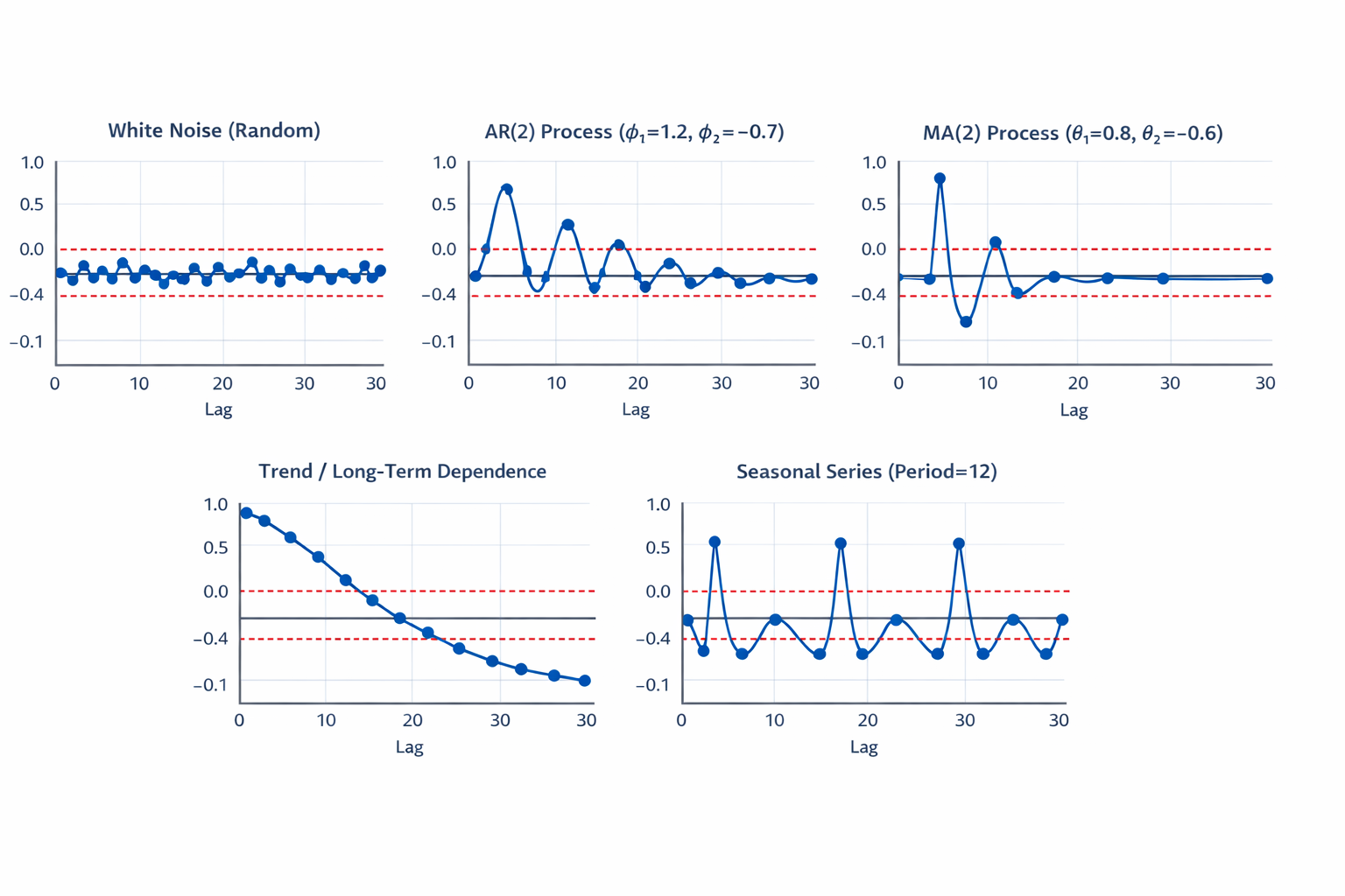
Example Correlogram
| Model | Purpose | Components / Formulation | Use / Notes |
|---|---|---|---|
| ARMA(p,q) | Stationary series | AR(p): | Short-term dependence modeling, requires stationarity |
| ARIMA(p,d,q) | Non-stationary series | Apply d-order differencing: | Removes trend, models short-term correlation |
| SARIMA(p,d,q) | Series with seasonality | Non-seasonal: ARIMA(p,d,q) | Models both trend and seasonal patterns; s = seasonal period |
| Modeling Steps |
| ||
Time Series Forecasting and Machine Learning
Time series forecasting can be converted into a machine learning problem to leverage the power of sequential models like RNNs and LSTMs.
1. Converting Time Series to ML Problem
- Supervised learning formulation:
Predict future values using past observations as features. - Sliding window approach:
Input: [X_{t-n}, X_{t-n+1}, ..., X_{t-1}]
Output: X_t
Multi-Step Forecasting Strategies
When forecasting beyond a single time step (), the complexity of the model increases as it must account for accumulating uncertainty and the lack of observed ground truth for future inputs. There are two primary architectural approaches, supplemented by robust feature engineering.
The Direct Method
In this approach, you develop a unique, independent model for each specific lead time in your forecast horizon.
- Mechanism: To forecast steps ahead, you train separate models. Model 1 is trained to predict using , Model 2 is trained to predict using , and so on.
- Pros: Prevents Error Accumulation, as each model is optimized for its specific target horizon without relying on previous (potentially noisy) predictions.
- Cons: High computational overhead (training models) and a lack of temporal coherence between predicted steps.
The Recursive (Iterative) Method
This method utilizes a single model trained for one-step-ahead prediction () and applies it sequentially to reach the desired horizon.
- Mechanism: The prediction for is treated as an "observed" value and fed back into the model as an input to predict .
- Pros: Computationally efficient (only one model required) and maintains a consistent internal logic across the entire forecast path.
- Cons: Error Propagation. Any bias or variance in the first prediction is compounded in every subsequent step, often leading to rapid performance degradation over long horizons.
Advanced Feature Engineering
To maximize the accuracy of either strategy, the stochastic process must be enriched with contextual features beyond simple historical values.
-
Temporal Dependencies (Lags): Incorporating previous observations () to capture the internal Autocorrelation of the series. This is the foundation of AR-based logic.
-
Window Statistics (Rolling Transforms): Utilizing Rolling Means or Exponentially Weighted Moving Averages (EWMA) to capture local trends and volatility changes, providing the model with a sense of "momentum."
-
Cyclical Time Features: Encoding calendar information (Hour of day, Day of week, Month) using Sine/Cosine Transformations: . This ensures the model understands that "Hour 23" is chronologically close to "Hour 0."
-
Exogenous Variables: Integrating external drivers—such as marketing spend, weather indices, or economic indicators—that provide causal context that the univariate history cannot provide.
Recurrent Neural Networks
RNN Architecture
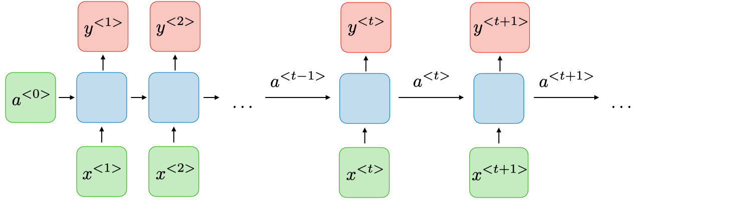
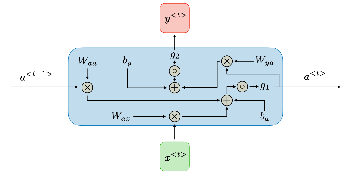
Recurrent Neural Networks (RNNs) are a class of neural networks that allow previous outputs to influence future computations via hidden states. They are commonly used for sequential data such as time series or text. For each timestep , the hidden state and the output are computed as follows:
- Hidden state:
- Output:
where:
- is the input at time
- is the hidden state at time
- is the output at time
- are weight matrices shared across all timesteps
- = biases
- = activation functions (e.g., tanh, ReLU, softmax)
RNN Architecture
| Advantages | Drawbacks |
|---|---|
• Possibility of processing input of any length | • Computation being slow |
Long Short-Term Memory (LSTM)
While classical models like ARIMA rely on linear combinations of past lags, the Long Short-Term Memory (LSTM) network is a specialized Recurrent Neural Network (RNN) architecture designed to learn long-term dependencies. It achieves this through a cell state regulated by a complex system of gates, effectively solving the vanishing gradient problem common in standard RNNs.
LSTM Architecture
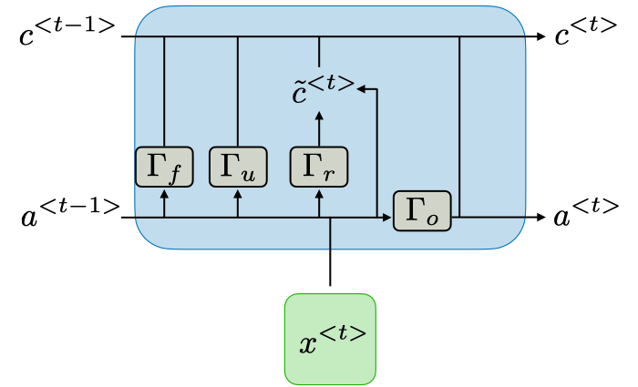
1. The Core Architecture
As shown in the architectural diagram, an LSTM unit at time step processes three distinct signals: the current input (), the previous hidden state (), and the previous cell state ().
The Gating Mechanisms
The unit contains four neural network layers (represented by the blocks), each acting as a filter for information flow:
- Forget Gate (): Examines and to decide which information from the previous cell state is no longer relevant and should be removed (multiplied by a value near 0).
- Update/Input Gate (): Determines which parts of the new information are worth storing.
- Candidate State ( or ): Creates a vector of new values that could be added to the state.
- Output Gate (): Controls which parts of the cell state are output to the hidden state (), which then serves as the short-term memory and the basis for the current prediction.
2. Mathematical State Transitions
The power of the LSTM lies in its ability to modify the Cell State () via additive operations, allowing gradients to flow through time without being drastically scaled.
Updating the Long-Term Memory
The new cell state is calculated by combining the "filtered" old memory with the "filtered" new candidate information:
Updating the Short-Term Memory
The hidden state is updated by passing the new cell state through a non-linear function and multiplying it by the output gate's result:
3. Practical Advantages in Time Series
LSTMs are particularly effective for univariate time series that contain:
- Non-linear dependencies that classical linear models (ARIMA) cannot capture.
- Variable length lags where the significant past event happened at an irregular interval.
- Complex seasonality where multiple cycles (daily, weekly, yearly) overlap in non-additive ways.
References
[1] C. Chatfield and H. Xing, The Analysis of Time Series: An Introduction with R, 7th ed. Boca Raton, FL, USA: CRC Press, 2019.
[2] J. Brownlee, Deep Learning for Time Series Forecasting: Predict the Future with MLPs, CNNs and LSTMs in Python, v1.1 ed. Machine Learning Mastery, 2018.
[3] M. Joseph, Modern Time Series Forecasting with Python: Explore industry-ready forecasting solutions from stock methods to deep learning. Birmingham, UK: Packt Publishing, 2022.