
Lecture 11
Contents
- TinyML: Machine Learning at the Edge
- 2. From Cloud ML to TinyML
- 3. Edge Computing Architecture
- 4. TinyML: Technical Fundamentals
- 6. TinyML Development Workflow
- 7. Applications & Use Cases
- 8. Challenges & Future Directions
- Development Complexity: The Expertise Gap
- The Power-Performance Tradeoff
- Model Updates and Lifelong Learning
- Looking Ahead: The Future of TinyML
- Career Opportunities
- Summary & Key Takeaways
- Resources for Continued Learning
TinyML: Machine Learning at the Edge
What is TinyML?
Imagine you have a smoke detector in your home. Traditional smoke detectors work by sensing particles in the air, but they can't distinguish between smoke from your burnt toast and smoke from an actual fire. They're dumb sensors that trigger on any smoke. Now imagine a smoke detector that can actually smell the difference—one that uses a tiny neural network to classify the type of smoke and only sounds the alarm for genuine fires. This is TinyML.
TinyML, which stands for Tiny Machine Learning, represents a revolutionary convergence of two powerful technologies: machine learning and embedded systems. It's the art and science of running sophisticated machine learning models on microcontrollers—the same tiny, low-power chips that run your thermostat, your fitness tracker, or the sensors in your car.
Definition
The formal definition from the TinyML Foundation describes it as "a fast-growing field of machine learning technologies and applications >including hardware, algorithms and software capable of performing on-device sensor data analytics at extremely low power, typically in the mW >range and below." But what does this really mean for us as engineers and what makes it so transformative?
At its core, TinyML is about bringing intelligence to the very edge of our computing infrastructure—not to powerful servers in the cloud, not even to relatively capable edge computers like Raspberry Pis, but all the way down to the smallest, most power-constrained devices imaginable. We're talking about devices that run on batteries for months or even years, devices with memory measured in kilobytes rather than gigabytes, and devices that cost just a few dollars.
The Fundamental Characteristics
-
To truly understand TinyML, we need to grasp its defining characteristics. First and foremost is ultra-low power consumption. While your laptop might consume 50 watts and a data center GPU might consume 300 watts or more, TinyML devices operate in the milliwatt to microwatt range. To put this in perspective, imagine a coin cell battery—the kind you might find in a watch. A TinyML device can run continuously on such a battery for years. This isn't just an incremental improvement; it's a complete paradigm shift that enables entirely new applications.
-
The second characteristic is the tiny footprint. We're working with devices that have just kilobytes to a few megabytes of memory. Your smartphone has 4-8 gigabytes of RAM; a typical TinyML device like an Arduino Nano has just 256 kilobytes of flash memory and 32 kilobytes of RAM. That's roughly 100,000 times less memory than your phone! This severe constraint forces us to be incredibly creative and efficient in how we design and deploy our models.
-
Third is on-device inference. Unlike cloud-based systems where your data travels to a remote server for processing, TinyML performs all computation locally on the device itself. The sensor data never needs to leave the device unless you specifically want it to. This local processing has profound implications for privacy, latency, and system reliability.
-
Finally, TinyML enables real-time response measured in milliseconds rather than seconds. There's no network latency, no waiting for a cloud response. When a TinyML device detects an event, it can act on it immediately.
Why TinyML Matters: A Deeper Look
Let's explore why TinyML is so important through a concrete scenario. Imagine you're developing a fall detection system for elderly care. This is a real-world application where the design decisions we make can literally save lives.
The Traditional Cloud Approach:
In a cloud-based system, you would place sensors on the elderly person that constantly stream accelerometer and gyroscope data to a smartphone. The smartphone would then transmit this data over WiFi or cellular to a cloud server running sophisticated machine learning models. The cloud would analyze the movement patterns, detect if a fall has occurred, and send an alert back through the network to emergency services or family members.
This approach has several serious problems. First, there's latency. Even with a fast internet connection, the round-trip time for data to travel to the cloud and back is typically 200-500 milliseconds. When someone has fallen and might be injured, every second counts. Second, what happens when there's no WiFi? Many elderly people fall in their bathrooms or basements where network coverage might be spotty. Third, there's the privacy concern: do we really want to send continuous accelerometer data from someone's body to a cloud server? This is personal health information that many people would prefer to keep private. Fourth, the constant data transmission drains the smartphone battery quickly, requiring daily charging—which defeats the purpose if the person forgets to charge it. Finally, there are the ongoing costs of cloud computing and data transmission that add up month after month.
The TinyML Approach:
Now consider the TinyML alternative. We place a tiny, lightweight sensor directly on the person's clothing or as a pendant. This sensor contains a microcontroller running a trained fall detection model. The device constantly monitors movement patterns, but all processing happens locally. When the model detects a fall signature—the characteristic pattern of sudden acceleration followed by impact—it immediately triggers an alert through a simple radio signal or the person's phone.
The response time is now under 10 milliseconds. There's no dependence on WiFi or cellular coverage—the detection happens regardless. All movement data stays on the device, preserving privacy completely. The tiny battery can last for months without recharging. And there are no ongoing cloud costs. This is the power of TinyML.
The Converging Trends
TinyML exists at the intersection of several powerful technological trends, each of which has been developing for decades.
First, there's the relentless progress of Moore's Law applied to microcontrollers. Modern microcontrollers pack dramatically more computing power into the same tiny packages. A modern ARM Cortex-M4 microcontroller, despite being designed for ultra-low power operation, has more computing power than the computers that guided Apollo missions to the moon. This computational capability, combined with specialized hardware accelerators for machine learning operations, makes it feasible to run neural networks on devices that cost just a few dollars.
Second, we've seen revolutionary advances in machine learning algorithms. The same models that once required powerful GPUs can now be compressed and optimized to run on tiny devices with minimal accuracy loss. Techniques like quantization, where we reduce the precision of numbers from 32-bit floating point to 8-bit integers, can shrink models by 75% while losing less than 1% accuracy. Pruning techniques can remove up to 90% of a model's parameters while maintaining performance. These aren't just engineering tricks—they represent fundamental insights into how neural networks work and what information is truly essential for making accurate predictions.
Third, the software tools have matured dramatically. Just a few years ago, deploying machine learning on a microcontroller required deep expertise in embedded systems, careful manual optimization, and a lot of trial and error. Today, frameworks like TensorFlow Lite for Microcontrollers, Edge Impulse, and specialized libraries handle much of this complexity automatically. A student with basic programming knowledge can now deploy a neural network to a microcontroller in an afternoon.
Finally, there's enormous market demand. The Internet of Things is exploding—we're heading toward a world with hundreds of billions of connected devices. But sending all the data from these devices to the cloud for processing is neither economically viable nor technically feasible. TinyML offers a solution: bring the intelligence to the device, process data locally, and only transmit what's truly necessary. This shift from "sense and transmit" to "sense, process, and selectively transmit" is transforming IoT from a data problem into an intelligence solution.
The Market Reality
The numbers tell a compelling story. Industry analysts project the TinyML market will grow from around 2.5 billion by 2030. This isn't just venture capital hype—it represents real deployment of TinyML solutions in industries from healthcare to manufacturing to agriculture.
Consider the sheer scale: there are expected to be over 250 billion IoT devices deployed by 2030. If even 10% of these devices incorporate TinyML capabilities, that's 25 billion intelligent edge devices making real-time decisions without cloud connectivity. Each of these devices represents a point where data doesn't need to flow to the cloud, where privacy is preserved by default, where latency is measured in microseconds rather than seconds, and where battery life is measured in years rather than hours.
The economic implications are equally profound. Companies deploying TinyML solutions report bandwidth savings of 90-95% compared to traditional IoT architectures. They eliminate or dramatically reduce cloud computing costs. They achieve faster response times that enable new applications. And they do all this while improving privacy and security.
2. From Cloud ML to TinyML
Understanding the Spectrum
To truly appreciate TinyML, we need to understand where it fits in the broader landscape of machine learning deployment. Think of machine learning deployment as existing along a spectrum—a continuum from unlimited computing resources in the cloud to severely constrained resources at the extreme edge.
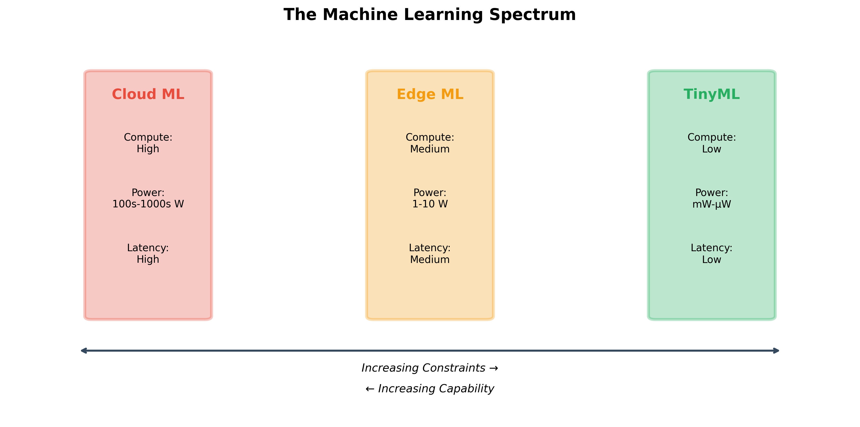
Figure 1:Spectrum of ML Solutions
At one end of this spectrum sits cloud machine learning. Imagine the data centers that power services like Google Search, Netflix recommendations, or ChatGPT. These facilities house thousands of powerful GPUs, each consuming hundreds of watts of power. They have effectively unlimited memory and storage, measured in terabytes. They can perform trillions of operations per second. A single training run for a large language model might use the equivalent energy of several households for an entire year. This is machine learning at its most powerful—and most resource-intensive.
When we deploy models in the cloud, we make implicit tradeoffs. We accept network latency of hundreds of milliseconds because we gain access to enormous computational power. We accept ongoing costs of tens or hundreds of thousands of dollars per month for cloud computing. We accept that data must travel potentially thousands of miles from the sensor to the data center and back. For applications like web search or recommendation systems, these tradeoffs make perfect sense. The computational complexity is enormous, batch processing is acceptable, and the marginal cost per query is tiny when amortized across billions of users.
In the middle of our spectrum sits edge machine learning. This is the domain of devices like smartphones, Raspberry Pis, and NVIDIA Jetson boards. A modern smartphone has a remarkably capable neural processing unit (NPU) that can perform billions of operations per second. Your iPhone's Face ID, for instance, runs sophisticated neural networks entirely on-device. The smartphone strikes a balance: it has gigabytes of memory, moderate power consumption (charging daily is acceptable for most users), and processing capabilities that would have been supercomputer-level just two decades ago.
Edge ML represents a sweet spot for many applications. Your phone can recognize faces, transcribe speech, or identify objects in photos without sending data to the cloud. The latency is low enough for real-time interaction, the privacy is better than cloud-based approaches, and the user experience is seamless. However, edge ML still requires significant power—your phone might last a day or two on a charge, but not weeks or months. It still needs substantial memory measured in gigabytes. And it still costs hundreds of dollars per device.
Entering the TinyML Domain
Now we reach the extreme edge of our spectrum: TinyML. Here, the constraints are severe almost unimaginable if you're used to working with traditional computing systems. Let's make these constraints concrete.
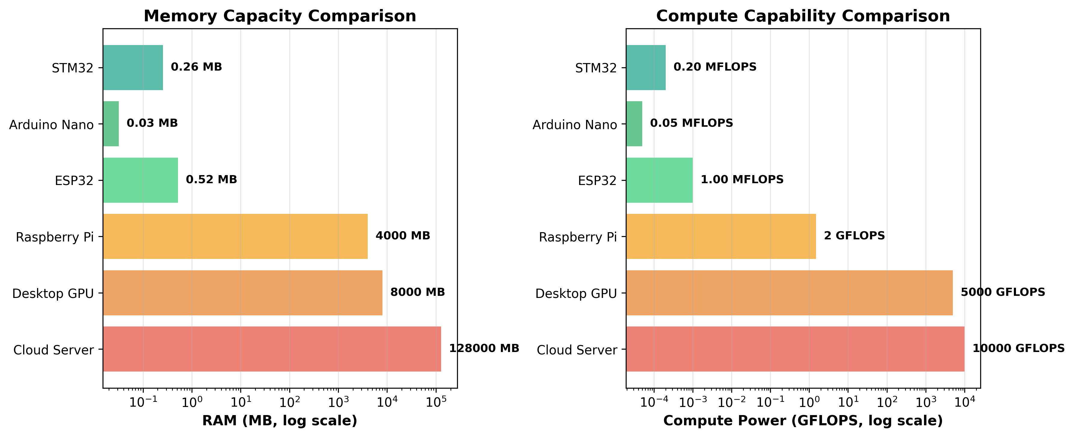
Figure 2:Hardware Comparison
A typical cloud server might have 128 gigabytes of RAM. A smartphone has 8 gigabytes. A Raspberry Pi has 4 gigabytes. An ESP32 microcontroller—a common choice for TinyML applications—has 520 kilobytes. An Arduino Nano has just 32 kilobytes of RAM. To put this in perspective, this paragraph you're reading right now, as plain text, would consume most of an Arduino Nano's entire memory!
The computational differences are equally dramatic. A modern data center GPU can perform 10 trillion floating-point operations per second (10 TFLOPS). A smartphone might manage 1-2 TFLOPS. A Raspberry Pi achieves about 1.5 gigaflops (GFLOPS). An ESP32? About 1 megaflop (MFLOP)—that's 10 million times slower than the data center GPU.
Yet somehow, remarkably, we can still run useful machine learning models on these constrained devices. How is this possible?
The Power Dimension
Perhaps the most dramatic difference lies in power consumption, and this is where TinyML truly shines. Let's think about this through the lens of battery life, because that's what ultimately matters for real-world deployments.
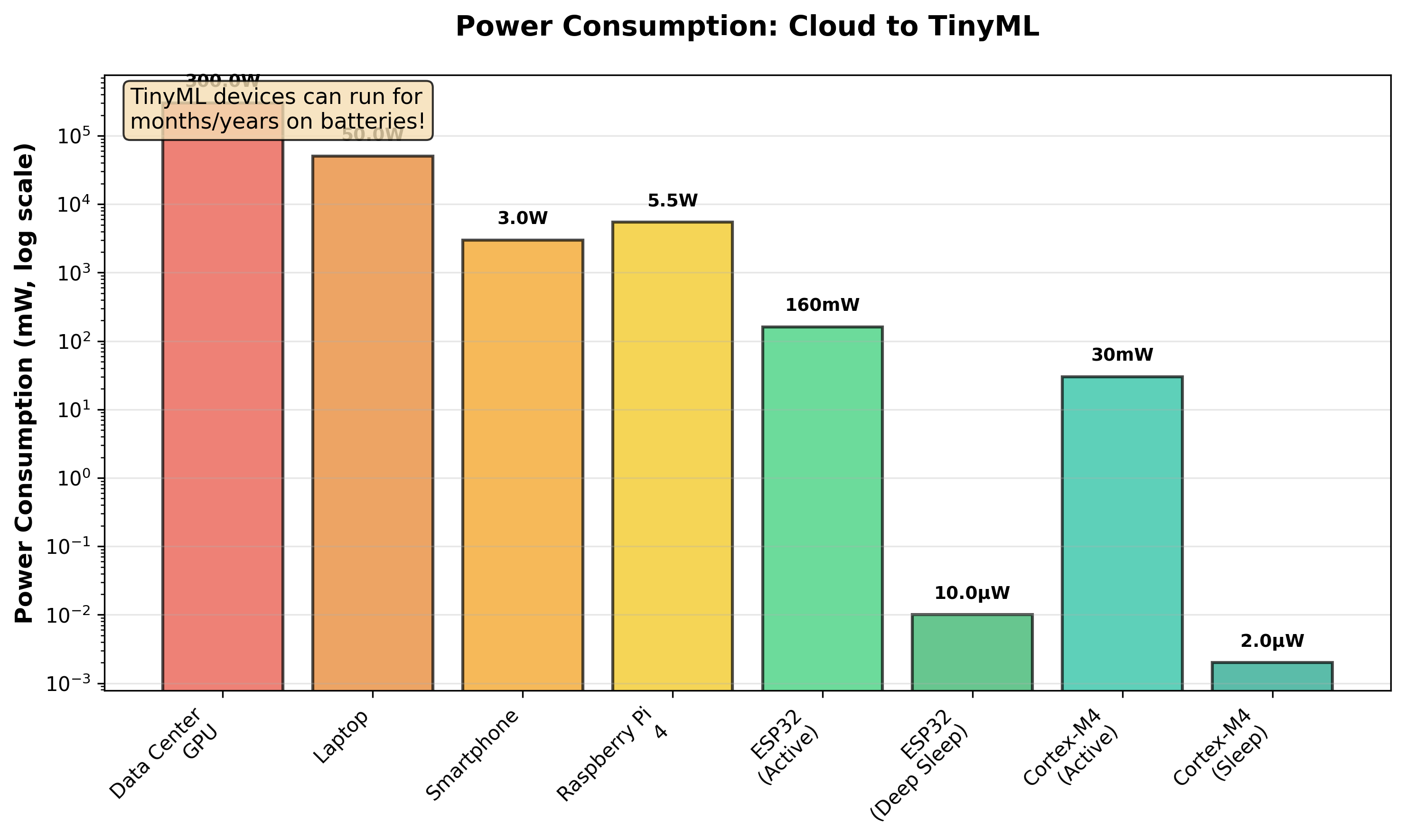
Figure 3: Power consumption
Imagine you have a standard coin cell battery—a CR2032, the kind you might find in a car key fob. This battery stores about 1,000 milliamp-hours (mAh) of charge at 3 volts, giving us roughly 3,000 milliwatt-hours of energy.
A data center GPU consuming 300 watts would drain this battery in about 36 seconds. Not particularly useful!
A laptop consuming 50 watts would last about 3 minutes.
A smartphone running machine learning might consume 3 watts during active processing, giving us perhaps an hour of operation—though in reality, smartphones have much larger batteries.
A Raspberry Pi 4 consuming 5.5 watts would last about 30 minutes on our tiny coin cell.
Now here's where it gets interesting. An ESP32 microcontroller, when actively running TinyML inference, typically consumes about 160 milliwatts. On our coin cell battery, this would last about 18-20 hours of continuous operation. But ESP32s don't need to run continuously—they can sleep between inferences. In deep sleep mode, an ESP32 consumes just 10 microwatts. At this rate, it could run for over 30 years on a single coin cell!
In practice, a TinyML device that wakes up once per second to check for events, runs inference for 10 milliseconds, then goes back to sleep can easily last 1-5 years on a small battery. This is fundamentally different from any other computing paradigm we've discussed. It enables "deploy and forget" scenarios where you can place a sensor, and it will simply work for years without maintenance.
A Thought Experiment: Keyword Spotting
Let's make this concrete with a real-world example: always-on voice activation (like "Hey Siri" or "OK Google").
The Cloud Approach:
To implement "always-on" wake word detection using the cloud, your device would need to constantly stream audio to a remote server. At typical audio quality (16kHz, 16-bit), this is about 32 kilobytes per second or 2.5 gigabytes per day per device. For 100 million devices, that's 250 petabytes of data per day flowing to the cloud! The energy cost of transmitting this data would drain a smartphone battery in hours. The privacy implications of constantly streaming audio from homes and pockets to corporate servers are obviously troubling. The cloud computing costs would be astronomical. And the latency—the time between speaking and getting a response—would be 200-500 milliseconds even in ideal conditions.
The Edge Approach (Smartphone):
Modern smartphones use a dedicated low-power chip to listen for wake words. This chip consumes perhaps 100-200 milliwatts while listening. It can identify the wake word locally and only then activate the main processor and network connectivity. This is much better than the cloud approach, but it still drains the battery—wake word detection is one reason smartphone batteries rarely last more than a day or two.
The TinyML Approach:
Now imagine a truly tiny implementation. A microcontroller running a quantized neural network can detect wake words while consuming just 1-2 milliwatts of power. At this level, a small battery can power the device for months or years. All processing is local—no audio ever leaves the device unless the wake word is detected. The latency is under 10 milliseconds. And the hardware cost is under $5 per device.
This isn't a theoretical comparison—this is how products like Amazon Echo Dot or Google Nest Mini actually work. They use dedicated TinyML chips for wake word detection, only engaging their more powerful processors and network connections after detecting "Alexa" or "Hey Google."
Making the Tradeoffs
So when should you use cloud ML, edge ML, or TinyML? The answer depends on your constraints and requirements.
Choose cloud ML when you need massive computational power for complex tasks, when you're okay with network latency, when you have reliable connectivity, when you're processing batch data rather than real-time streams, and when power consumption and device cost aren't primary concerns. Cloud ML is perfect for training large models, for applications like web search or recommendation engines, and for analytics on historical data.
Choose edge ML when you need more power than TinyML can provide but want to avoid cloud latency and costs. This is the sweet spot for smartphone applications, autonomous vehicles, or industrial gateways that need to process data from multiple sensors. Edge devices can run medium-sized models, handle multi-modal inputs (combining camera, microphone, and sensors), and provide good user experiences without cloud dependencies.
Choose TinyML when power consumption is critical, when you need battery operation for months or years, when privacy is paramount (data must never leave the device), when network connectivity is unreliable or unavailable, when you need sub-10-millisecond latency, or when device cost must be minimal. TinyML is perfect for wearables, environmental sensors, industrial IoT, wildlife monitoring, and any application where you deploy thousands or millions of sensors.
The beautiful thing is that these approaches can work together. A TinyML device might perform initial filtering and anomaly detection locally, an edge gateway might aggregate and process data from hundreds of TinyML devices, and the cloud might handle model training and long-term analytics. The key is choosing the right level for each task.
3. Edge Computing Architecture
The Three-Tier Architecture
To understand where TinyML fits in modern systems, we need to understand the architecture of edge computing. Think of it as a three-tier pyramid, where intelligence and processing happen at different levels based on the requirements of speed, power, and computational complexity.
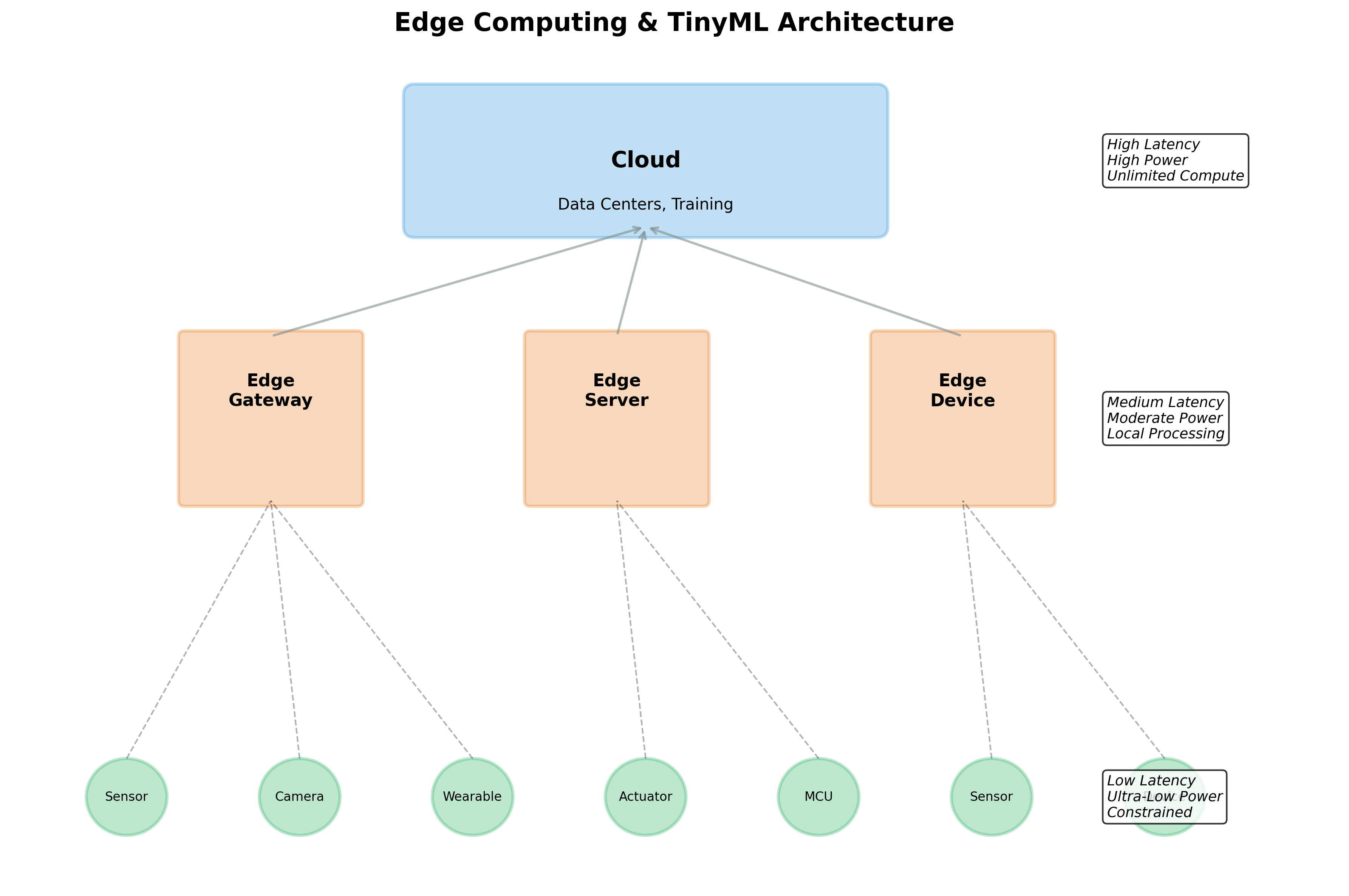
The Cloud Tier: The Brain
At the top of our pyramid sits the cloud layer—the centralized brain of the system. This is where the heavy lifting happens: training machine learning models on massive datasets, performing complex analytics on historical data, and generating insights that require looking at patterns across thousands or millions of devices. The cloud has unlimited computational resources and storage, but it's distant from the sensors and actuators actually interacting with the physical world.
Think of the cloud as a master chef who creates recipes and occasionally checks in on how the kitchen is running. The chef doesn't need to be involved in every single dish being cooked, but they design the processes, update the recipes based on feedback, and maintain overall quality standards.
In our TinyML systems, the cloud typically handles model training, periodic model updates pushed to edge devices, dashboard and visualization for human operators, and long-term trend analysis and reporting. A key insight: the cloud sees aggregated, processed data rather than raw sensor feeds. Instead of receiving megabytes of raw sensor data, it might receive a few kilobytes of processed insights and alerts.
The Edge Gateway: The Coordinator
The middle tier consists of edge gateways or edge servers. These are moderately powerful computing devices—think Raspberry Pis, industrial PCs, or specialized edge computing appliances. They sit between the cloud and the sensor devices, acting as coordinators and aggregators.
Using our kitchen analogy, edge gateways are like sous chefs. They supervise a station, aggregate work from multiple junior cooks (the TinyML sensors), handle some processing that's too complex for the sensors but doesn't need to go to the cloud, and communicate with the head chef when necessary.
Edge gateways typically aggregate data from hundreds or thousands of TinyML sensors, perform protocol translation (converting between sensor protocols and cloud APIs), handle local caching and buffering when cloud connectivity is interrupted, run medium-complexity models that are too large for microcontrollers, and filter and compress data before sending it to the cloud.
The edge gateway is optional in some architectures but crucial in others. For a single smart home device, you might not need a gateway—the TinyML sensor can communicate directly with the cloud when needed. But for an industrial facility with thousands of sensors, edge gateways become essential for managing the complexity and bandwidth requirements.
The TinyML Tier: The Front Line
At the base of our pyramid, closest to the physical world, sits the TinyML layer—potentially thousands or millions of tiny, intelligent sensors. These are the eyes, ears, and decision-makers operating in real-time at the point of data collection.
In our kitchen analogy, TinyML devices are like line cooks with specialized training. They know exactly how to prepare their specific dishes without constant supervision. They can handle routine tasks independently and only alert the sous chef when something unusual happens.
TinyML devices perform real-time sensing and immediate inference on sensor data, make split-second decisions without consulting the cloud or edge gateway, filter data at the source by only transmitting relevant events or anomalies, and preserve privacy by processing sensitive data locally without storing or transmitting it.
The key architectural insight is that TinyML devices are smart filters. Instead of sending raw data upstream, they apply intelligence to extract only what's meaningful. A camera might capture 30 frames per second, generating gigabytes of data per hour. But a TinyML vision system might recognize that nothing interesting is happening and send zero bytes upstream for hours, then send a single alert when it detects an anomaly.
Real-World Example: Smart Building
Let's make this architecture concrete with a detailed example of a smart building system that uses TinyML to optimize energy usage while maintaining occupant comfort.
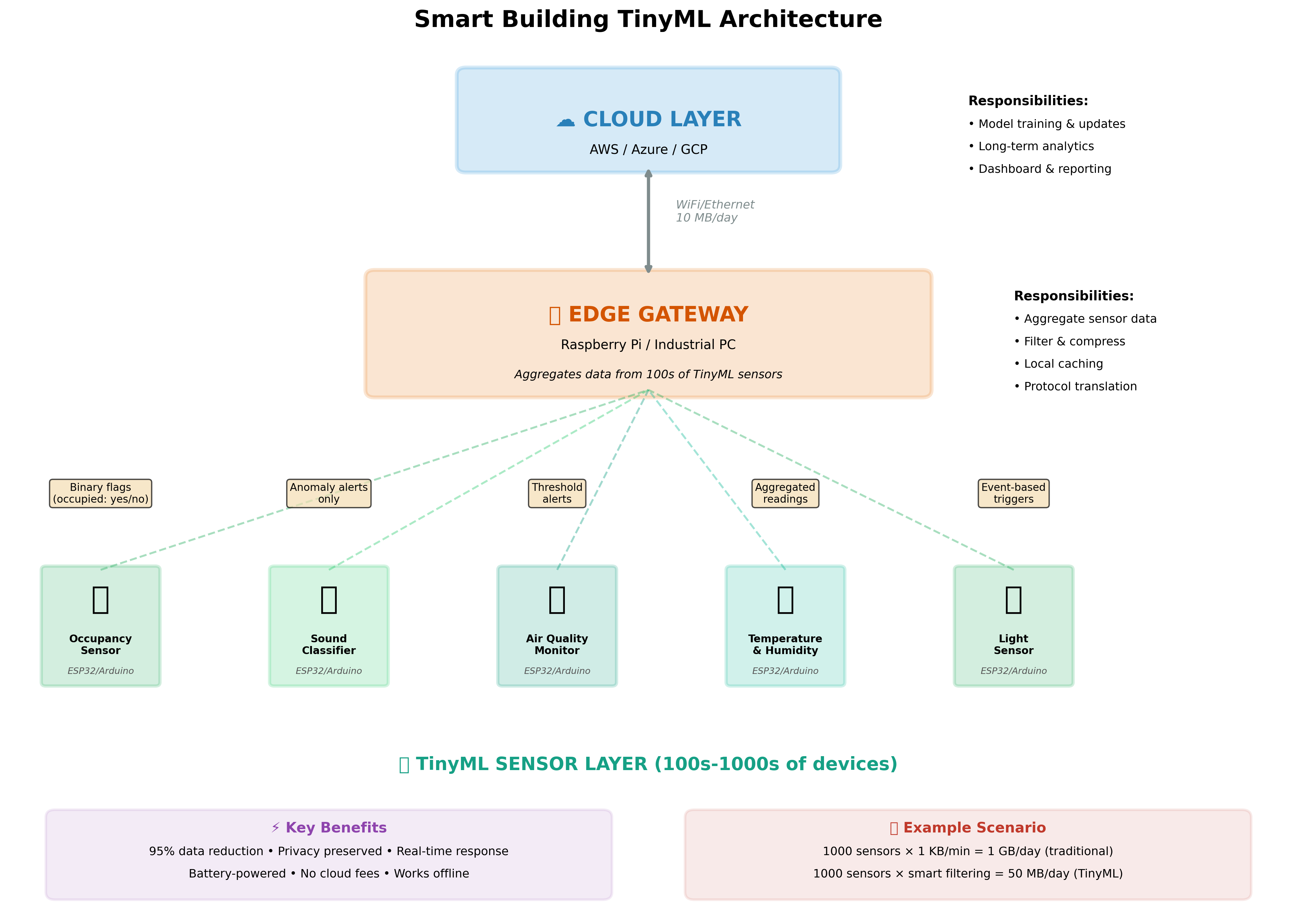
Smart Building Architecture
Imagine a modern office building with 50 floors and 5,000 occupants. Our goal is to minimize energy consumption while ensuring people are comfortable—proper temperature, good air quality, and adequate lighting.
The TinyML Sensor Layer:
Throughout the building, we deploy 1,000 tiny, battery-powered sensor nodes. Each node costs about $20 and contains an ESP32 microcontroller along with various sensors. Let's look at what different sensors do:
Occupancy sensors use passive infrared (PIR) sensors combined with a tiny neural network that can distinguish between humans, pets, and cleaning robots. Traditional PIR sensors can't tell the difference—they just detect movement. Our TinyML version analyzes movement patterns: humans move in characteristic ways, stop to work at desks, and move purposefully between locations. Pets move erratically. Cleaning robots follow predictable paths.
Each sensor runs inference every second. When it detects human occupancy, it sends a simple binary flag to the edge gateway: "Room 415 occupied: yes." That's it—just one bit of information, or in practice, a few bytes for the message packet. When the room becomes unoccupied, another message: "Room 415 occupied: no." Compare this to traditional approaches that might stream video continuously or capture images every few seconds, generating megabytes of data per hour with significant privacy implications.
Sound classifiers listen to ambient audio using tiny microphones, running a convolutional neural network that can identify different types of sounds. They can distinguish normal office sounds (typing, talking, footsteps) from anomalies (breaking glass, smoke alarms, shouting). Under normal conditions, they send nothing upstream—zero bytes of data. They might update a local counter of activity level every minute, transmitting one number.
But when they detect glass breaking or a smoke alarm, they immediately send an alert. Crucially, they never record or transmit actual audio. The neural network processes audio in real-time and only outputs classification labels. An intruder could physically capture a sensor and would find no recorded audio, no raw data—just the trained model weights. This is privacy by architecture.
Air quality monitors continuously measure CO₂, volatile organic compounds (VOCs), temperature, and humidity. A TinyML model running on each sensor learns the normal baseline for its specific location and can predict upcoming air quality issues based on patterns. For instance, if CO₂ levels start rising in a pattern consistent with a meeting room filling up, the sensor can alert the HVAC system proactively rather than reactively.
The models only transmit data when meaningful changes occur. Instead of sending 1,440 readings per day (one per minute), they might send 10-20 events: "CO₂ rising above threshold," "returning to normal," "unusual VOC detected." This reduces data transmission by 98% while providing better, more actionable information.
Temperature and humidity sensors with TinyML can do something clever that traditional sensors cannot: they can predict thermal comfort rather than just measuring temperature. Thermal comfort is subjective and depends on temperature, humidity, air movement, and even occupant activity level. A TinyML model trained on historical data and occupant feedback can learn to predict when people are likely to be uncomfortable and adjust HVAC proactively. These sensors might update their predictions every 5 minutes but only alert when actual adjustment is needed.
Light sensors monitor ambient illumination and use TinyML to optimize lighting based on natural light, time of day, and occupancy. They can detect when a room has sufficient natural light and automatically dim or turn off artificial lights. They learn patterns—certain rooms might get strong afternoon sun and need shading rather than artificial light. Each sensor makes autonomous decisions about its local lighting zone while coordinating with neighbors through the edge gateway.
The Edge Gateway Layer:
On each floor, we have an edge gateway—a small industrial PC running Linux. This gateway collects data from 20-30 TinyML sensors on its floor, aggregates the occupancy data to create a floor-level occupancy map, coordinates between sensors, and runs more complex models that require data from multiple sensors.
For example, the edge gateway might notice that the east side of a floor is consistently warmer in the morning (sun exposure) while the west side is warmer in the afternoon. It can adjust HVAC zones accordingly. It might detect that certain conference rooms are heavily used on Tuesday mornings and pre-condition them. These insights require looking at patterns across multiple sensors over time—something too complex for individual TinyML devices but not requiring cloud resources.
The edge gateway also handles local caching. If cloud connectivity is interrupted, it continues operating the building using local intelligence. It buffers any data that needs to go to the cloud and uploads it when connectivity returns.
Each floor gateway might receive 50-100 kilobytes per hour from its TinyML sensors (after the sensors have already done 95% filtering). It processes this data, extracts insights, and sends perhaps 1-2 kilobytes per hour up to the cloud—a further 50x reduction.
The Cloud Layer:
The cloud receives aggregate data from all 50 floor gateways. It sees building-wide patterns: overall energy consumption, occupancy trends over weeks and months, and long-term optimization opportunities. It uses this data to retrain and improve the TinyML models running on sensors, performs energy consumption optimization across the whole building, generates reports for building managers, and integrates with other building systems.
The cloud might receive 100 kilobytes per hour from a building with 1,000 sensors. In a traditional IoT architecture without TinyML, those same sensors generating 1 MB per hour each would be sending 1 terabyte per hour—a reduction of 10 million times!
The Economic Impact:
Let's calculate the bandwidth savings. Traditional approach: 1,000 sensors sending 1 MB/hour = 1 TB/hour = 24 TB/day. At typical cloud ingestion costs of $0.10 per GB, that's $2,400 per day or $876,000 per year just for data ingestion.
TinyML approach: After sensor-level filtering, edge aggregation, and compression, we send perhaps 2.4 GB per day total. Cost: $240 per year—a 99.97% reduction!
This doesn't even account for the reduced cloud computing costs (less data to process), the reduced network infrastructure costs, the improved privacy and security, or the faster response times that enable better building control.
4. TinyML: Technical Fundamentals
The Constraint Triangle
When working with TinyML, you're constantly navigating what I call the "constraint triangle"—three interconnected limitations that define the boundaries of what's possible: memory, compute power, and energy. These aren't independent variables; they're deeply connected, and improving one often means compromising on another.
Think of it like planning a backpacking trip where you can only carry a certain weight. You need shelter, food, and water, but you can't bring everything you want. If you bring more food (more memory for your model), you might have less capacity for water (less memory for activation buffers). If you want to hike faster (higher performance), you'll burn through your food supplies quicker (more power consumption). The art of TinyML is finding the right balance for your specific journey.
Memory: Your Canvas
Memory is perhaps the hardest constraint because it's absolutely fixed. A microcontroller with 256 KB of flash memory cannot magically have more. You can optimize your code, compress your model, and be clever with data structures, but you cannot exceed the physical memory available.
Memory in microcontrollers comes in two primary forms, and understanding the distinction is crucial. Flash memory is non-volatile—it retains its contents when power is removed. This is where your program code and trained model weights live. It's relatively abundant (modern microcontrollers might have 512 KB to 2 MB of flash) but slower to access and cannot be written to during normal program execution.
SRAM (Static Random Access Memory) is volatile—it loses its contents when power is removed. It's fast, can be read from and written to freely, but is precious and scarce. A typical TinyML microcontroller might have only 32 KB to 256 KB of SRAM. This is where your program's variables, stack, and crucially, the activation buffers for neural network computation must live.
Here's why SRAM is often the limiting factor: when running a neural network, you need to store intermediate results (activations) as you process each layer. Consider a simple convolutional layer that takes a 96x96 RGB image as input and outputs 32 feature maps of size 48x48. Even if we quantize to 8-bit integers, those output activations require 96×96×32 = 294,912 bytes—that's 288 KB just for one layer's output! On a device with 256 KB total SRAM, this is impossible.
This is why TinyML practitioners obsess over activation memory. The model weights might fit comfortably in flash, but the runtime memory requirements for activations can make or break your deployment. We use techniques like in-place operations (reusing activation buffers), careful operator ordering, and architecture choices specifically designed to minimize activation memory.
Compute: Your Processing Power
Compute power in microcontrollers is measured very differently than in desktop or server systems. We don't talk about GFLOPS (billions of floating-point operations per second); we talk about MIPS (millions of instructions per second) or, for machine learning specifically, MOPS (millions of operations per second).
A modern ARM Cortex-M4 microcontroller running at 64 MHz might achieve 80 MIPS at peak. Compare this to a desktop CPU achieving tens of thousands of MIPS, or a GPU achieving millions of MIPS, and you start to appreciate the challenge. For TinyML, we might achieve 1-10 MOPS when running neural network inference.
What does this mean in practice? Let's say you have a neural network with 1 million multiply-accumulate (MAC) operations—a small model by modern standards. On a desktop GPU, this might take microseconds. On a microcontroller, it might take 100-1000 milliseconds. For many applications, especially those requiring real-time response to sensor inputs, this is the difference between "works" and "doesn't work."
This is why we care so much about model size and efficiency. Each MAC operation in your model translates directly to computation time. Reducing parameters by 10x might reduce inference time by 10x, which could be the difference between meeting your latency requirements or not.
Power: Your Battery Budget
Power consumption ties everything together because it directly affects how long your device can operate on a battery. Every computation costs energy. Every memory access costs energy. Even keeping the device powered on in idle state costs energy.
Modern microcontrollers are remarkably efficient, but the physics of computation sets fundamental limits. A typical rule of thumb: each million operations per second costs about 1 milliwatt. So if you're running inference that requires 10 million operations and you do this once per second, you're consuming about 10 milliwatts on average.
But here's where it gets interesting: microcontrollers can sleep. Deep sleep modes consume microwatts or even nanowatts—thousands of times less than active processing. The key to ultra-low-power TinyML is spending as much time as possible sleeping and waking up only when necessary.
Consider a TinyML audio classification system listening for specific sounds. One approach: sample audio continuously, run inference continuously. This might consume 100 milliwatts—giving you perhaps 10 hours on a small battery. Better approach: use a simple energy detector (which costs almost no power) to detect when audio is present, wake up the ML model only when sounds are detected, process the audio, classify it, then immediately return to sleep. Average power: perhaps 1 milliwatt, giving you 1,000 hours (6 weeks) on the same battery.
The art of low-power TinyML is understanding these sleep/wake cycles and orchestrating them effectively.
Memory Architecture Deep Dive
Let's get very concrete about memory management because this is where many TinyML projects succeed or fail. I'll use a real example: deploying a keyword spotting model to an Arduino Nano 33 BLE Sense.
The Arduino Nano 33 has 1 MB of flash and 256 KB of SRAM. Seems like a lot, right? Let's see where it goes:
Flash Budget (1 MB total):
- Arduino bootloader and core libraries: ~150 KB
- TensorFlow Lite for Microcontrollers library: ~200 KB
- Our application code (sensor handling, communication, etc.): ~100 KB
- Model weights: We have about 550 KB available
- Reserve for overhead and future updates: ~100 KB
So we have about 450-550 KB for our actual model weights. If we use 8-bit quantization (1 byte per weight), this means our model can have about 450,000-550,000 parameters. A reasonable-sized model for keyword spotting might have 200,000-300,000 parameters, so we're okay on flash.
SRAM Budget (256 KB total):
- Stack (for function calls, local variables): ~8 KB
- Heap (for dynamic allocation): ~20 KB
- Static variables and globals: ~10 KB
- TensorFlow Lite interpreter overhead: ~20 KB
- Activation buffers: Here's the critical part!
We have about 200 KB available for activation buffers. Now, keyword spotting typically works on 1-second windows of audio at 16 kHz sampling rate. That's 16,000 samples. If we store them as 16-bit integers, that's 32 KB just for the input buffer.
The model processes this through several layers. A typical architecture might include:
- Convolutional layer: outputs 40x10x8 = 3,200 bytes
- Another conv layer: outputs 40x10x16 = 6,400 bytes
- Flatten and dense layers: outputs might be 4,000 bytes
If we're not careful, the total activation memory could be 50-80 KB. Added to our input buffer and other requirements, we're using perhaps 120-150 KB of our 200 KB budget. This works, but there's not much margin for error.
This is why TensorFlow Lite for Microcontrollers has an "arena" allocator—a clever system that reuses memory buffers between layers. As soon as a layer finishes computing and its outputs are consumed by the next layer, its activation buffer can be recycled. This typically cuts activation memory by 50-70%.
The Reality of Microcontroller Platforms
Let's look at specific hardware platforms to make this concrete. These are the actual devices you'll work with in your projects.
Arduino Nano 33 BLE Sense: The Learning Platform
This is probably the most popular board for learning TinyML, and for good reason. Based on the Nordic nRF52840 chip with an ARM Cortex-M4 core running at 64 MHz, it includes an impressive array of sensors built right onto the board: a 9-axis IMU (accelerometer, gyroscope, magnetometer), digital microphone, temperature and humidity sensor, barometric pressure sensor, ambient light sensor, and color sensor.
For your first TinyML project, this board is ideal because everything is integrated. You don't need to wire up sensors; you can immediately start collecting data and training models. The 256 KB of SRAM is generous enough for learning but constrained enough that you'll understand the memory challenges. At around $30, it's affordable for educational purposes.
The limitations? The 64 MHz clock means inference can be slow for larger models. Battery life, while good, isn't in the "years" category. And there's no WiFi, so connectivity requires pairing with a smartphone or computer.
ESP32: The Versatile Workhorse
The ESP32 has become the default choice for IoT applications, and it's also excellent for TinyML. With two Xtensa LX6 cores running at up to 240 MHz, 520 KB of SRAM, and 4 MB of flash, it has significantly more computational power than the Arduino Nano. The built-in WiFi and Bluetooth make connectivity trivial.
What makes ESP32 particularly interesting for TinyML is its deep sleep capability. In active mode with WiFi, it might consume 160 milliwatts. In deep sleep, just 10 microwatts. This dramatic difference enables applications that wake up periodically to perform inference, transmit results if needed, and then sleep for hours or days.
For your object detection projects, the ESP32-CAM variant is particularly useful. It includes a small camera module and all the connectivity you need for about $6—remarkably cost-effective. The catch? The camera consumes significant power, so battery life won't be measured in months, but for many applications, days of operation is sufficient.
STM32 Family: The Professional Choice
STMicroelectronics' STM32 family represents the professional end of microcontrollers used in TinyML. The STM32L4 series is optimized for ultra-low power, while the STM32H7 series offers high performance with ARM Cortex-M7 cores running at 480 MHz.
These aren't hobby boards; they're what goes into production devices. They offer hardware accelerators for certain operations, sophisticated power management, and extensive peripheral support. They're also more complex to work with, typically requiring professional development tools.
For academic projects, STM32 boards like the Nucleo series offer a middle ground: professional-grade hardware at educational prices with good development tool support.
Neural Networks for TinyML
Now that we understand our constraints, let's talk about the neural network architectures that actually work within these constraints.
Remember, the goal isn't to run the latest cutting-edge model. The goal is to run the simplest model that solves your problem adequately. This is a fundamental mindset shift from conventional machine learning.
MobileNet: Designed for Efficiency
MobileNet, developed by Google, introduced the concept of depthwise separable convolutions—a clever reformulation of standard convolutions that dramatically reduces both parameter count and computation.
In a standard convolution, you convolve a filter of size K×K across C input channels to produce one output channel. For N output channels, this requires K×K×C×N multiplications. For a 3×3 convolution with 32 input channels and 64 output channels, that's 3×3×32×64 = 18,432 multiplications.
Depthwise separable convolutions split this into two steps. First, apply a depthwise convolution: use a 3×3 filter on each input channel independently, requiring K×K×C operations. Then apply a pointwise convolution: use 1×1 convolutions to combine channels, requiring C×N operations. Total: (K×K×C) + (C×N) = (3×3×32) + (32×64) = 288 + 2,048 = 2,336 operations—nearly 8× fewer!
The beautiful thing about depthwise separable convolutions is that they lose very little accuracy compared to standard convolutions. In many cases, the accuracy drop is less than 1% while achieving this dramatic reduction in computation and parameters.
For TinyML, MobileNetV2 and MobileNetV3 are common starting points. They provide pre-trained models that can be fine-tuned for your specific application, then quantized and compressed for deployment.
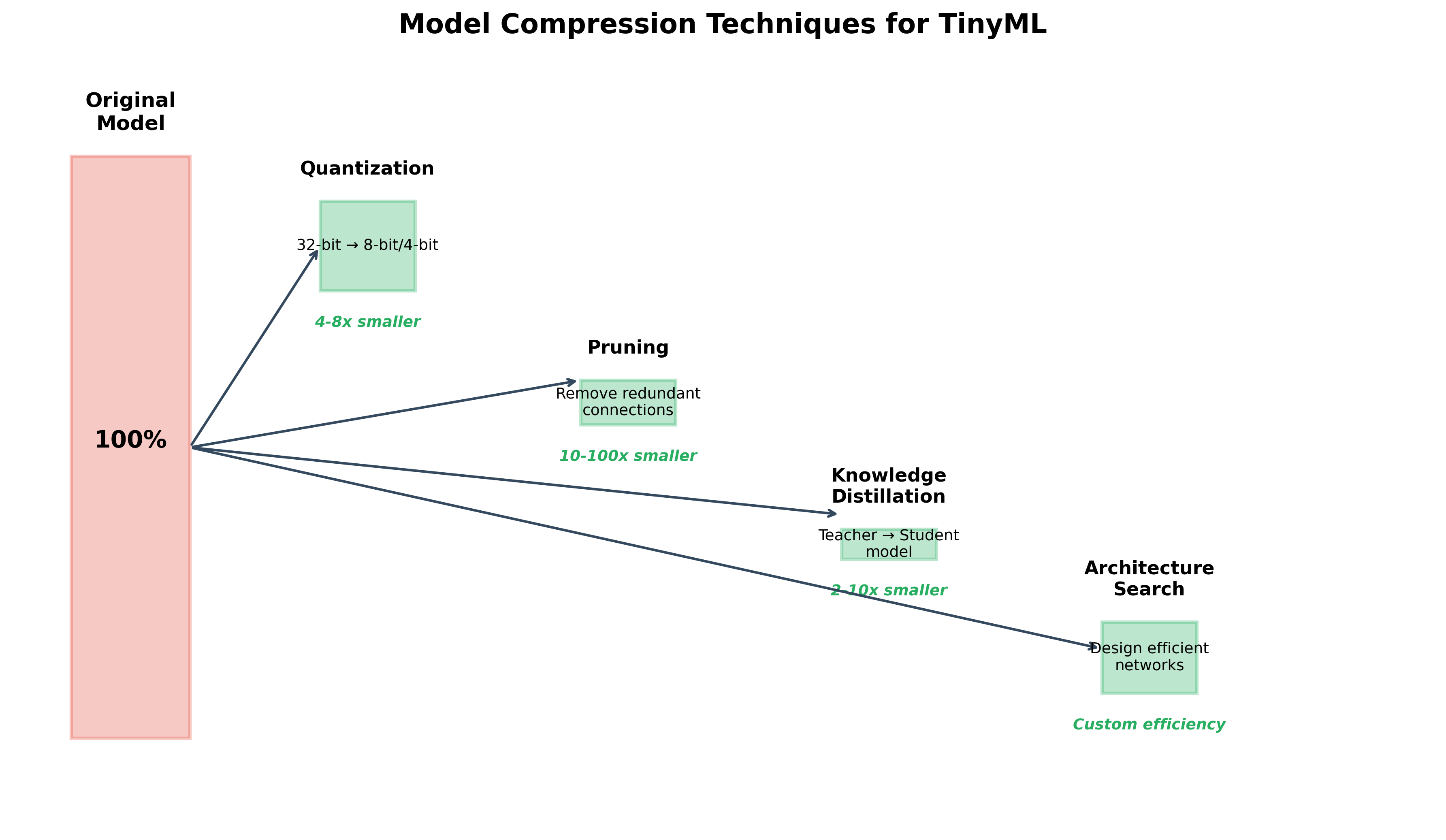
Quantization: Making Models Tiny
Quantization is perhaps the single most important technique in TinyML, so let's really understand how it works and why it's so powerful.
When you train a neural network in TensorFlow or PyTorch, by default, every number is a 32-bit floating-point value. This includes all model weights, all activations, all intermediate calculations. A 32-bit float can represent numbers from about -3.4×10³⁸ to +3.4×10³⁸ with about 7 decimal digits of precision.
But here's the key insight: neural networks don't actually need this level of precision. Through extensive research, it's been shown that for inference (running a trained model), 8-bit integers are usually sufficient. Sometimes even 4-bit integers work!
How Quantization Works:
The basic idea is to map the range of float values to the range of integer values using a scale factor and zero point. Mathematically:
real_value = scale * (quantized_value - zero_point)
For example, if your weights range from -0.5 to +0.5, you can map them to the 8-bit integer range of -128 to +127. The scale would be 0.5/128 ≈ 0.00391, and the zero point would be 0.
When you quantize a trained model, you compute the scale and zero point for each layer based on the actual range of values in that layer. Then you convert all the float32 weights to int8, storing the scale and zero point as metadata.
The Benefits:
The memory savings are immediate and dramatic: int8 uses 1 byte per value versus 4 bytes for float32—a 4× reduction. A model with 100,000 parameters shrinks from 400 KB to 100 KB.
The computational speedup is even better. Integer arithmetic is much faster than floating-point arithmetic on microcontrollers. Many microcontrollers don't even have hardware floating-point units; they must emulate floating-point operations in software, which can be 10-100× slower. With quantized models, inference speed often improves by 3-5×.
The power savings follow from the speed improvement. Faster inference means less time with the processor active, which means lower average power consumption.
The Accuracy Trade-off:
Quantization does reduce accuracy, but usually very little. Post-training quantization (where you take a trained float32 model and quantize it directly) typically loses 0.5-2% accuracy. Quantization-aware training (where you simulate quantization during training so the model learns to be robust to quantization errors) often loses less than 0.5% accuracy—sometimes even gaining accuracy!
For many TinyML applications, this trade-off is completely acceptable. A keyword spotting model that goes from 96% accuracy to 94.5% accuracy is still highly usable. An anomaly detector that goes from 98% to 97% is fine.
5. Model Compression & Optimization
(20 minutes)
Think of model compression as packing for a trip. You start with everything you might possibly need—a suitcase full of clothes, gadgets, toiletries. But you're flying on a budget airline with strict weight limits. You need to get your essentials into a tiny carry-on bag. Model compression is the art of taking a large, accurate neural network and systematically removing everything that isn't absolutely essential, while maintaining the model's ability to make good predictions.
Model Compression
Quantization: The Detail Lens
We've touched on quantization, but let's go deeper into why it works so remarkably well. The key insight comes from understanding what neural networks actually learn.
When you train a neural network, you're essentially learning a very complex function that maps inputs to outputs. This function is defined by millions or billions of parameters—the weights and biases. But here's the surprising thing: the exact values of these parameters don't matter nearly as much as their relationships to each other.
Think of it this way: imagine you're trying to recognize faces. The exact numerical value of a particular weight might be 0.34719284. But what really matters is that this weight is larger than its neighbor (say, 0.23841) and smaller than another neighbor (say, 0.51223). The relative magnitudes and signs of weights are what create the patterns that the network uses to make decisions.
Quantization preserves these relationships while using far less precision. When we quantize from float32 to int8, we're saying: "We don't need to know that this weight is exactly 0.34719284. Knowing that it's approximately 0.347 is good enough." We lose some precision, but we retain the essential structure of the function the network has learned.
Advanced Quantization Techniques:
Modern TinyML development often uses several quantization strategies simultaneously:
Per-layer quantization recognizes that different layers need different levels of precision. The first layers of a neural network, which process raw input data, might need more precision. The final layers, which produce classification scores, might work fine with aggressive quantization. By tuning the quantization parameters layer-by-layer, we can often improve accuracy compared to uniform quantization.
Mixed precision quantization takes this further. Some layers might use 8-bit integers, others 4-bit, and critical layers might even stay at 16-bit or float32. The goal is to use the minimum precision needed for each layer while meeting our overall size and accuracy targets.
Calibration is crucial for good quantization. When you quantize a model, you need to know the range of values to expect for weights and activations. Poor calibration leads to clipping (where values exceed your quantized range) and poor accuracy. Good practice is to run your model on a representative dataset during quantization, observing the actual ranges of values, and using these ranges to set optimal scale factors.
Pruning: The Sculptor's Approach
If quantization is about reducing precision, pruning is about reducing quantity. Pruning removes entire parameters or structures from the neural network, creating a sparser model.
The inspiration for pruning comes from neuroscience. The human brain at birth has roughly 100 billion neurons and 1 quadrillion synapses (connections). But during childhood and adolescence, the brain actively prunes connections—eliminating up to 50% of synapses in some regions. This pruning actually improves brain function, removing weak or redundant connections and strengthening the important pathways.
Neural networks exhibit similar behavior. After training, many connections have very small weights—effectively contributing little to the network's decisions. Pruning identifies and removes these weak connections.
The Pruning Process:
Start with a trained model that achieves good accuracy. Analyze the weight magnitudes across the network. Sort all weights by absolute value. Remove the smallest weights—typically starting with the bottom 20-30% by magnitude. Fine-tune the remaining network to recover lost accuracy. Gradually increase pruning percentage while monitoring accuracy.
Here's what's remarkable: you can often remove 70-90% of weights with less than 1-2% accuracy loss! A model with 1 million parameters might work nearly as well with just 100,000-300,000 parameters.
Structured vs. Unstructured Pruning:
Unstructured pruning removes individual weights. This gives maximum flexibility—you can keep exactly the weights that matter most. However, the resulting sparse model (lots of zeros scattered throughout) doesn't actually run faster on most hardware unless you use specialized sparse matrix operations.
Structured pruning removes entire channels, filters, or neurons. This is less flexible but much more practical. If you remove an entire filter from a convolutional layer, the resulting model is truly smaller and faster—no need for specialized sparse operations.
For TinyML, structured pruning is usually more useful because microcontrollers don't typically have optimized sparse matrix libraries. Better to have a genuinely smaller model than a large model full of zeros.
Pruning Example:
Let's make this concrete. Imagine you have a simple convolutional neural network for gesture recognition:
- Conv layer: 3×3×16 filters = 432 parameters
- Conv layer: 3×3×32 filters = 4,608 parameters
- Dense layer: 128×64 = 8,192 parameters
- Dense layer: 64×4 = 256 parameters
- Total: ~13,500 parameters
After training, analysis shows the first conv layer has 3 filters (out of 16) with very small weights across all positions. We remove these filters entirely:
- Conv layer: 3×3×13 filters = 351 parameters (19% reduction)
The second conv layer can be reduced from 32 to 24 filters:
- Conv layer: 3×3×24 filters = 3,456 parameters (25% reduction)
The first dense layer is the largest, and we find we can reduce it to 128×48:
- Dense layer: 128×48 = 6,144 parameters (25% reduction)
New total: ~10,200 parameters (24% reduction)
After fine-tuning for 10-15 epochs, accuracy drops from 94.3% to 93.8%—a very acceptable trade-off for a 24% reduction in model size and corresponding speedup in inference.
Knowledge Distillation: The Mentor Method
Knowledge distillation is one of my favorite techniques because it's based on such an elegant idea: the best way to train a small model isn't necessarily to train it directly on your data. Instead, train a large, accurate model first (the "teacher"), then use this teacher to train a smaller "student" model.
Why does this work? The teacher model has learned rich representations and subtle patterns in the data. When it makes predictions, it doesn't just output hard labels (cat vs. dog); it outputs probabilities that contain much more information. A teacher might say "I'm 99% confident this is a cat, 0.5% dog, 0.3% rabbit, 0.2% other." These "soft labels" capture the model's uncertainty and the relationships between classes.
The student model learns not just from the ground truth labels but from the teacher's soft predictions. In a sense, the student is learning not just what the right answers are, but how to think about the problem—the same way a human student learns more from a good teacher's explanations than from just memorizing answers.
The Distillation Process:
Train a large teacher model on your full dataset. This model should achieve the best possible accuracy—don't worry about size or speed. Design a much smaller student architecture (perhaps 10-100× smaller). Generate soft labels by running the teacher on your training data. Train the student model using a combination of hard ground truth labels and teacher soft labels.
The training objective combines two losses:
- Loss compared to ground truth (traditional training)
- Loss compared to teacher predictions (distillation)
You control the balance with a temperature parameter and a weighting factor. Typically, you weight the distillation loss heavily (80-90%) because that's where the student learns the nuanced patterns.
Practical Example:
Let's say you're building a visual wake-up gesture system for a smart home—wave your hand and lights turn on. You collect 10,000 images of hand gestures from various angles, distances, and lighting conditions.
Teacher model: Use MobileNetV2 as a base, fine-tune on your data. The model has 3.5 million parameters and achieves 97% accuracy. It's too large for your ESP32-CAM.
Student model: Design a tiny custom CNN with just 50,000 parameters—70× smaller. When trained directly on the dataset, it achieves 91% accuracy. Not terrible, but not great.
With distillation: Train the same 50,000-parameter model using the teacher's soft labels. Final accuracy: 94.5%! You've retained most of the teacher's performance while using 70× fewer parameters.
This 3.5% accuracy improvement might seem small, but it's the difference between a frustrating user experience (failing to recognize gestures 9% of the time) and a delightful one (failing only 5.5% of the time).
Neural Architecture Search: The Automated Designer
Neural Architecture Search (NAS) flips the traditional approach to neural network design on its head. Instead of having a human expert design the architecture based on intuition and experience, we automate the search for optimal architectures.
For TinyML, this is particularly valuable because the constraints are so severe and interdependent. A human might design a model that fits in memory but is too slow, or is fast enough but uses too much power. NAS can explore thousands of possible architectures and find ones that meet all constraints simultaneously.
How NAS Works:
Define your constraints explicitly: maximum model size, maximum inference time, maximum power consumption. Define your search space: what types of layers are allowed, what sizes, what connections. Use automated search (reinforcement learning, evolutionary algorithms, or gradient-based methods) to explore architectures. Train each candidate architecture and evaluate it against constraints. Over many iterations, discover architectures that meet your specific requirements.
MCUNet: Purpose-Built for TinyML:
MCUNet, developed at MIT, is a NAS system specifically designed for microcontrollers. It jointly optimizes the neural network architecture and the inference engine (the code that actually runs the model). This co-design approach leads to architectures that are dramatically more efficient than human-designed networks for specific hardware platforms.
For instance, MCUNet can design a model for visual wake-word detection on an Arduino Nano that achieves 75% accuracy with inference time under 20ms—beating hand-designed networks that either had lower accuracy or higher latency.
Combining Techniques: The Complete Workflow
In practice, you rarely use just one compression technique. The best results come from combining multiple approaches in a systematic workflow:
Step 1: Start with an efficient architecture Begin with a baseline like MobileNetV2 or use NAS to find an architecture suited to your task and hardware.
Step 2: Train with quantization awareness Instead of training with float32 and quantizing afterward, simulate quantization during training. The model learns to be robust to quantization errors.
Step 3: Apply knowledge distillation If you have time and compute, train a larger teacher model first and use distillation. This typically improves the small model's accuracy by 2-5%.
Step 4: Structured pruning Remove entire channels or neurons that contribute little. This actually makes the model smaller and faster, not just sparser.
Step 5: Final quantization Convert the pruned model to int8 or even int4, using calibration on a representative dataset.
Step 6: Optimize the inference engine Use optimized kernels specific to your hardware platform. This can provide another 2-3× speedup.
Real Numbers from a Real Project:
Let me share results from an actual project: classifying bird species by their songs for wildlife monitoring.
Original model (MobileNetV2 base): 3.2 MB, 95.8% accuracy, 850ms inference time on ESP32
After efficient architecture search: 800 KB, 95.1% accuracy, 320ms inference
After quantization-aware training: 800 KB, 95.2% accuracy, 320ms inference
Quantize to int8: 200 KB, 94.6% accuracy, 95ms inference
Add structured pruning: 140 KB, 93.9% accuracy, 70ms inference
Final distillation pass: 140 KB, 94.4% accuracy, 70ms inference
Final result: We went from 3.2 MB to 140 KB (23× smaller), from 850ms to 70ms (12× faster), lost only 1.4% accuracy, and the model now fits comfortably on an ESP32 with plenty of room for other functionality. This is the power of systematically combining compression techniques.
6. TinyML Development Workflow
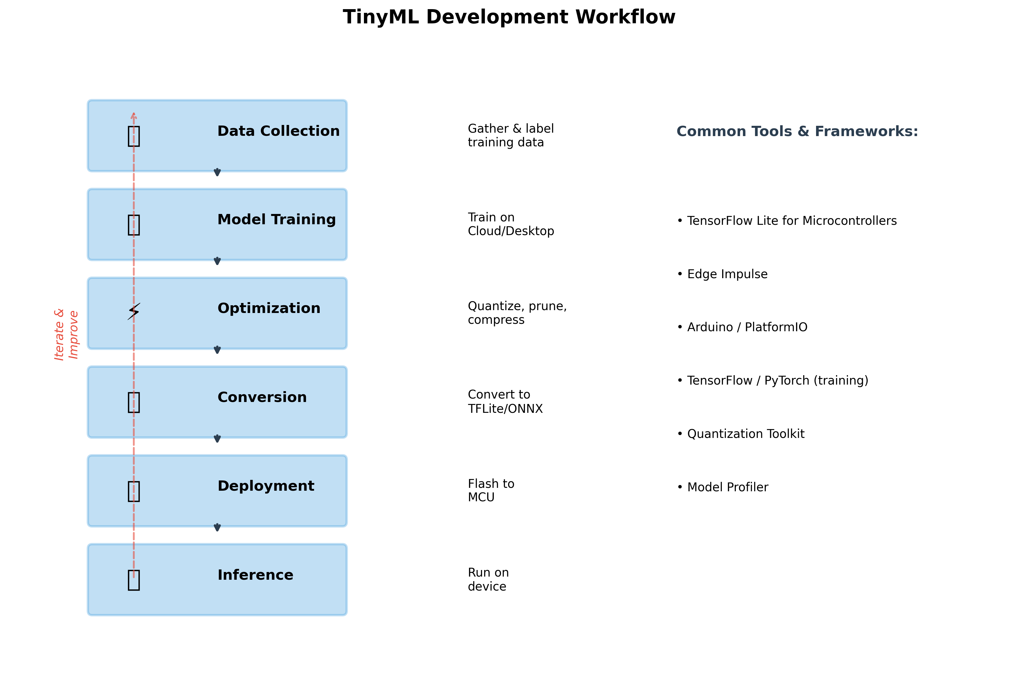
Developing a TinyML application is different from traditional software development or even traditional machine learning. You're working across multiple domains—embedded systems, machine learning, signal processing—and you need to understand how they interact. Let me walk you through the complete development workflow using a concrete example: building a gesture recognition system for smart home control.
TinyML Workflow
Step 1: Data Collection—The Foundation
Everything starts with data, but collecting data for TinyML has unique challenges. Unlike cloud ML where you might scrape millions of images from the internet, TinyML data must come from your actual target hardware. Why? Because sensors behave differently. An accelerometer on one board might have different noise characteristics than another. A microphone on your development board will capture audio differently than the microphone on your production device.
Our Gesture Recognition Example:
You're building a system that recognizes three gestures with a wrist-worn device: a wave (to turn on lights), a twist (to adjust brightness), and a double-tap (to turn off). The device uses a 6-axis IMU (accelerometer + gyroscope).
Start by wearing the Arduino Nano on your wrist and creating a simple data logging sketch. Press a button, perform the gesture, press the button again. The device saves one second of accelerometer and gyroscope data (6 channels × 50 samples per second = 300 values) along with the label.
But here's where many beginners make mistakes: they collect all the data themselves in one session. This creates a model that works great for you but fails for anyone else. Instead, you need diversity. Recruit 10-15 different people. Have them perform each gesture 30-50 times. Vary the conditions: dominant hand, non-dominant hand, sitting down, standing up, different speeds, with distractions.
After a few hours of collection, you have approximately 1,500 gesture samples (3 classes × 50 repetitions × 10 people). Save this data in a simple format—CSV files work fine. Each row: timestamp, ax, ay, az, gx, gy, gz, label.
The time investment in collecting good data pays enormous dividends later. A model trained on diverse, high-quality data might achieve 92% accuracy. The same model trained on narrow, poor-quality data might achieve only 75% accuracy—no amount of model architecture tweaking will fix this.
Step 2: Model Training—Start Simple
Now you're ready to train a model. For TinyML, always start with the simplest model that might possibly work. Resist the temptation to immediately jump to complex architectures.
For our gesture data:
Your input is 300 values (6 channels × 50 time steps). Your output is 3 classes (wave, twist, double-tap). A reasonable starting architecture:
import tensorflow as tf
from tensorflow import keras

model = keras.Sequential([
    # Reshape input to [batch, timesteps, channels]
    keras.layers.Reshape((50, 6), input_shape=(300,)),

    # Simple 1D CNN to extract temporal features
    keras.layers.Conv1D(8, kernel_size=3, activation='relu'),
    keras.layers.MaxPooling1D(2),

    keras.layers.Conv1D(16, kernel_size=3, activation='relu'),
    keras.layers.MaxPooling1D(2),

    # Flatten and classify
    keras.layers.Flatten(),
    keras.layers.Dense(16, activation='relu'),
    keras.layers.Dropout(0.2),
    keras.layers.Dense(3, activation='softmax')
])

model.compile(
    optimizer='adam',
    loss='sparse_categorical_crossentropy',
    metrics=['accuracy']
)
This model has about 3,000 parameters—quite small. Train it for 50 epochs with validation split:
history = model.fit(
    X_train, y_train,
    epochs=50,
    batch_size=32,
    validation_split=0.2,
    callbacks=[
        keras.callbacks.EarlyStopping(patience=10, restore_best_weights=True)
    ]
)
After training, you achieve 88% validation accuracy. Not perfect, but a solid start. The model is only 12 KB in float32 format.
The key principle: start simple and only add complexity if needed. Many students immediately jump to models with hundreds of thousands of parameters, which then don't fit on their target hardware. Better to start small and gradually increase capacity if accuracy isn't sufficient.
Step 3: Optimization—Making It Fit
Now comes the crucial step: converting your float32 model to a quantized int8 model suitable for deployment. This is where TensorFlow Lite shines.
import numpy as np

# Convert to TFLite with quantization
converter = tf.lite.TFLiteConverter.from_keras_model(model)
converter.optimizations = [tf.lite.Optimize.DEFAULT]

# Provide representative dataset for calibration
def representative_dataset():
    # Use a subset of training data
    for i in range(100):
        yield [X_train[i:i+1].astype(np.float32)]

converter.representative_dataset = representative_dataset

# Full integer quantization
converter.target_spec.supported_ops = [tf.lite.OpsSet.TFLITE_BUILTINS_INT8]
converter.inference_input_type = tf.int8
converter.inference_output_type = tf.int8

# Convert
tflite_model = converter.convert()

# Save
with open('gesture_model.tflite', 'wb') as f:
    f.write(tflite_model)

print(f"Original model: {model.count_params() * 4 / 1024:.1f} KB")
print(f"Quantized model: {len(tflite_model) / 1024:.1f} KB")
Output:
Original model: 12.0 KB
Quantized model: 3.2 KB
The quantized model is 3.7× smaller! Now verify that accuracy hasn't degraded too much. Run inference on your validation set using the TFLite interpreter and check accuracy. In this case, accuracy drops from 88% to 86.5%—acceptable.
Step 4: Conversion to C Array
Microcontrollers don't have filesystems where you can load a .tflite file. Instead, we embed the model directly into the firmware as a C array.
# Convert .tflite to C array
xxd -i gesture_model.tflite > model_data.cc
This produces:
unsigned char gesture_model_tflite[] = {
  0x1c, 0x00, 0x00, 0x00, 0x54, 0x46, 0x4c, 0x33,
  0x00, 0x00, 0x12, 0x00, 0x1c, 0x00, 0x04, 0x00,
  // ... 3,200 more bytes ...
};
unsigned int gesture_model_tflite_len = 3276;
Step 5: Deployment—Writing the Firmware
Now you write the Arduino sketch that runs your model. This involves several components:
Setting up the TFLite interpreter:
#include <TensorFlowLite.h>
#include "model_data.h"  // Contains gesture_model_tflite

namespace {
  // TensorFlow Lite for Microcontrollers components
  const tflite::Model* model = nullptr;
  tflite::MicroInterpreter* interpreter = nullptr;
  TfLiteTensor* input = nullptr;
  TfLiteTensor* output = nullptr;

  // Memory allocation for model
  constexpr int kTensorArenaSize = 8 * 1024;  // 8KB working memory
  uint8_t tensor_arena[kTensorArenaSize];
}

void setup() {
  Serial.begin(115200);

  // Load model
  model = tflite::GetModel(gesture_model_tflite);

  // Set up operations resolver (which operations the model uses)
  static tflite::MicroMutableOpResolver<5> resolver;
  resolver.AddConv2D();
  resolver.AddMaxPool2D();
  resolver.AddFullyConnected();
  resolver.AddReshape();
  resolver.AddSoftmax();

  // Build interpreter
  static tflite::MicroInterpreter static_interpreter(
    model, resolver, tensor_arena, kTensorArenaSize);
  interpreter = &static_interpreter;

  // Allocate memory for tensors
  interpreter->AllocateTensors();

  // Get pointers to input and output tensors
  input = interpreter->input(0);
  output = interpreter->output(0);

  Serial.println("Model loaded successfully!");
}
Reading sensors and running inference:
void loop() {
  // Buffer for one second of IMU data
  static float sensor_buffer[300];
  static int buffer_index = 0;

  // Read IMU at 50 Hz
  if (millis() % 20 == 0) {  // Every 20ms = 50Hz
    // Read accelerometer and gyroscope
    float ax, ay, az, gx, gy, gz;
    IMU.readAcceleration(ax, ay, az);
    IMU.readGyroscope(gx, gy, gz);

    // Add to buffer
    sensor_buffer[buffer_index * 6 + 0] = ax;
    sensor_buffer[buffer_index * 6 + 1] = ay;
    sensor_buffer[buffer_index * 6 + 2] = az;
    sensor_buffer[buffer_index * 6 + 3] = gx;
    sensor_buffer[buffer_index * 6 + 4] = gy;
    sensor_buffer[buffer_index * 6 + 5] = gz;

    buffer_index++;

    // When buffer is full (1 second of data)
    if (buffer_index >= 50) {
      buffer_index = 0;

      // Copy to model input (with quantization)
      for (int i = 0; i < 300; i++) {
        // Quantize: real_value = scale * (quantized - zero_point)
        // So: quantized = real_value / scale + zero_point
        input->data.int8[i] = sensor_buffer[i] / input->params.scale +
                              input->params.zero_point;
      }

      // Run inference
      uint32_t start_time = micros();
      TfLiteStatus invoke_status = interpreter->Invoke();
      uint32_t inference_time = micros() - start_time;

      if (invoke_status == kTfLiteOk) {
        // Get results (dequantize output)
        float scores[3];
        for (int i = 0; i < 3; i++) {
          scores[i] = (output->data.int8[i] - output->params.zero_point) *
                      output->params.scale;
        }

        // Find highest score
        int predicted_class = 0;
        float max_score = scores[0];
        for (int i = 1; i < 3; i++) {
          if (scores[i] > max_score) {
            max_score = scores[i];
            predicted_class = i;
          }
        }

        // Only act if confidence is high
        if (max_score > 0.8) {
          String gestures[] = {"Wave", "Twist", "Double-tap"};
          Serial.print("Detected: ");
          Serial.print(gestures[predicted_class]);
          Serial.print(" (");
          Serial.print(max_score * 100);
          Serial.println("%)");
          Serial.print("Inference time: ");
          Serial.print(inference_time);
          Serial.println(" μs");

          // Perform action (turn on lights, adjust brightness, etc.)
          handleGesture(predicted_class);
        }
      }
    }
  }
}
Step 6: Testing and Iteration
Deploy to hardware and test thoroughly. This is where you discover the gap between simulation and reality.
Common issues and solutions:
Memory overflow: If you get memory errors, you probably underestimated the tensor arena size. Monitor actual memory usage and adjust kTensorArenaSize.
Slow inference: If inference takes too long, you need to simplify your model or optimize. Target for inference time under 100ms for interactive applications.
Poor accuracy on device: If accuracy is much worse on-device than in training, check your quantization. Make sure you're properly scaling input values. Consider collecting more on-device data.
High power consumption: Profile power usage. You might be running inference too frequently or not using sleep modes effectively.
The development cycle is inherently iterative. Expect to go through this loop multiple times: collect more data, retrain with different architectures, re-optimize, re-deploy, test, repeat.
7. Applications & Use Cases
Healthcare and Wearables: Saving Lives with Milliwatts
Healthcare represents one of the most impactful application areas for TinyML. The combination of privacy preservation, low power consumption, and real-time response makes TinyML ideal for continuous health monitoring.
Consider epilepsy monitoring. People with epilepsy can experience seizures with little warning, which can be dangerous if they're alone or engaged in activities like driving. Traditional approaches require expensive hospital monitoring or are too power-hungry for continuous use.
A TinyML approach uses a small wearable device with accelerometers and gyroscopes. The device learns the specific seizure patterns for an individual patient—each person's seizures have unique characteristics. When the model detects the characteristic movements associated with seizure onset, it can immediately alert caregivers or emergency services.
The device runs for weeks on a small battery. All processing happens locally, so there's no concern about transmitting sensitive health data to the cloud. The sub-second response time means alerts go out immediately, not after valuable minutes have passed. And the cost—perhaps $50 per device—makes it accessible to many more patients than thousand-dollar hospital monitoring systems.
Similarly, continuous glucose monitoring with predictive alerts has become transformative for diabetes management. TinyML models can analyze the trend of glucose levels and predict hypoglycemic episodes 30 minutes before they occur. This advance warning gives patients time to eat something, potentially preventing dangerous blood sugar crashes. Because all processing happens on a tiny device worn by the patient, battery life extends to weeks, and there's no need for constant smartphone connectivity.
Industrial IoT: From Reactive to Predictive
Manufacturing environments are perfect for TinyML because of the scale involved. A single factory might have thousands of motors, pumps, conveyor belts, and other equipment. Traditional monitoring approaches can't scale economically—you can't justify expensive monitoring systems for every motor.
TinyML changes this calculus. For $10-20 per sensor, you can deploy vibration monitoring on every critical piece of equipment. Each sensor runs a lightweight anomaly detection model trained on the normal vibration signature of that specific motor or pump. When vibration patterns change in ways that indicate bearing wear, misalignment, or impending failure, the sensor sends an alert.
The economic impact is substantial. Unplanned downtime in manufacturing costs hundreds or thousands of dollars per minute. Preventive maintenance based on calendar schedules means replacing parts that might still have months of life left. Predictive maintenance—replacing parts based on actual condition—optimizes both uptime and maintenance costs.
A mid-sized automotive parts manufacturer deployed TinyML vibration sensors on 500 motors. In the first year, they detected 23 impending failures with average advance warning of 3-4 days. Estimated savings from avoided downtime: over 2 million. Cost of the sensor deployment: about \15,000. The ROI speaks for itself.
Smart Buildings: Efficiency Through Intelligence
Office buildings represent massive energy consumption—in the US alone, commercial buildings account for nearly 40% of total energy use. Even modest efficiency improvements have huge impact.
Traditional building management systems are coarse-grained. They might control HVAC by zone, with perhaps 10-50 zones in a large building. But occupancy is highly variable: some areas are constantly full while others are rarely used. Some rooms get direct sunlight; others never do.
TinyML enables ultra-fine-grained building control. Instead of 50 zones, you might have 1,000 smart sensors providing room-level or even desk-level intelligence. Each sensor knows: Is this space occupied? What's the temperature and humidity? What's the CO₂ level? How much natural light is available?
The TinyML models run locally on each sensor, making autonomous decisions about lighting and HVAC in coordination with neighbors. The system learns patterns: this conference room is always used Tuesday mornings, so pre-condition it. This area gets afternoon sun, so close the blinds automatically. This section of the building empties after 5pm, so reduce HVAC to minimum.
Real-world deployments show 20-30% energy savings compared to traditional building management systems. For a large office building spending 200,000-$300,000 in savings every year—while improving occupant comfort through more responsive control.
Environmental Monitoring: Scaling Scientific Research
TinyML is democratizing environmental science by making large-scale sensor deployments economically feasible. Consider wildlife monitoring: traditionally, studying animal populations required expensive equipment and labor-intensive field work. You might deploy a few dozen camera traps or audio recorders, checking them monthly, and spending hundreds of hours manually reviewing footage.
TinyML audio classifiers can identify bird species by their calls, running continuously on solar-powered sensors for years. For the cost of one traditional field season with a team of researchers, you can deploy hundreds of TinyML sensors across a landscape, collecting data 24/7/365.
Researchers at Cornell studying nighttime bird migration deployed 150 TinyML audio sensors across New York state. Each sensor costs about $30, runs on solar power with battery backup, and classifies bird calls locally. The system has recorded millions of bird detections, providing unprecedented insight into migration patterns—data that would have been impossible to collect manually.
Similarly, monitoring streams and rivers for water quality traditionally requires either expensive laboratory analysis or limited grab samples. TinyML sensors with spectroscopic capabilities can monitor water continuously, detecting pollution events in real-time. When anomalies are detected, detailed data gets transmitted for analysis. Otherwise, the sensors operate autonomously, requiring minimal bandwidth.
The Common Thread
Across all these applications, several patterns emerge. TinyML works best when you need continuous monitoring but can't justify continuous transmission of data. It's ideal when privacy matters—processing locally protects sensitive information. It enables applications where battery life must extend to months or years. And it's perfect for deployments at scale, where the low cost per device makes thousands or millions of sensors economically viable.
8. Challenges & Future Directions
TinyML is an exciting field, but it's not without significant challenges. Understanding these challenges—and the emerging solutions—is crucial as you develop your own projects and perhaps contribute to advancing the field.
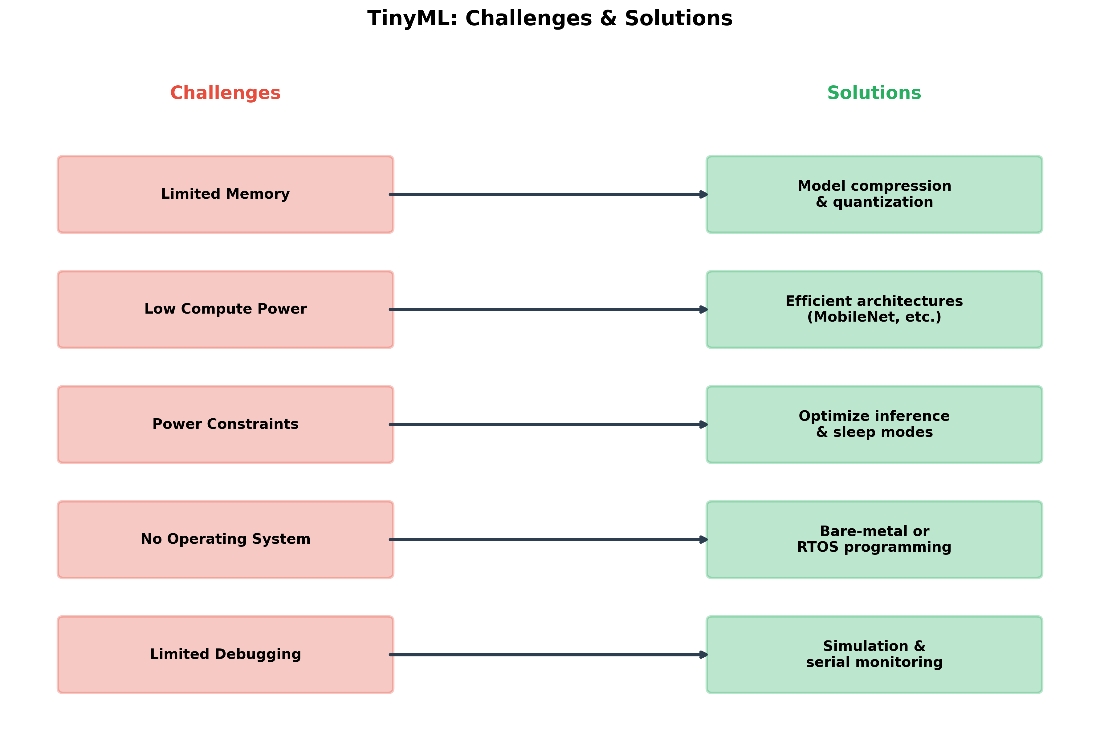
Challenges and Solutions
The Memory Wall
Perhaps the most fundamental challenge in TinyML is memory—both the amount available and the type. Unlike software development where you can often add more RAM, or cloud ML where memory is effectively unlimited, TinyML hardware has fixed, severe memory constraints.
The challenge isn't just total memory capacity; it's the split between Flash and SRAM. You might have 1 MB of Flash, which seems like enough for a model, but only 256 KB of SRAM. As we discussed earlier, activation memory—the intermediate values computed during inference—must fit in SRAM. A model might have modest parameter count but huge activation memory requirements, making it impossible to deploy.
Current solutions include in-place operations, where we reuse activation buffers; operator fusion, where multiple operations are combined to reduce intermediate storage; and careful architecture design to minimize peak activation memory. But these are workarounds, not solutions.
The real solution requires hardware innovation. Some new microcontrollers are adding small amounts of on-chip PSRAM (pseudo-static RAM), which provides more capacity while maintaining low power. Others incorporate specialized neural network accelerators with built-in memory management optimized for ML operations. The next generation of TinyML hardware will likely have more balanced memory architectures designed specifically for neural network inference.
Development Complexity: The Expertise Gap
Developing TinyML applications requires expertise across multiple domains: machine learning, embedded systems programming, signal processing, and often domain-specific knowledge (acoustics for audio applications, computer vision for visual applications, etc.). This is a lot to ask, and it creates a significant barrier to entry.
A mechanical engineer who understands vibration analysis might struggle with neural network training. A data scientist who can build excellent models might not understand microcontroller power management. Few people have the complete skill set needed.
This is where tools and platforms come in. Edge Impulse, SensiML, and similar platforms are abstracting away much of the complexity. They provide end-to-end workflows from data collection through deployment, with minimal coding required. While these tools don't eliminate the need for understanding the underlying concepts, they make it possible for domain experts to deploy TinyML without becoming experts in embedded systems or deep learning.
The future likely involves even more automation: models that design themselves for specific hardware targets, automated data collection strategies, and one-click deployment pipelines.
The Power-Performance Tradeoff
Even with all our optimization techniques, there's an inherent tradeoff between power consumption and model performance. More complex models provide better accuracy but consume more energy. Finding the sweet spot—the simplest model that achieves acceptable accuracy—requires careful tuning and often application-specific considerations.
Emerging hardware addresses this with specialized accelerators. Neural processing units (NPUs) designed specifically for ML operations can perform inference 10-100× more efficiently than general-purpose microcontroller cores. For example, a Cortex-M4 running a CNN might consume 100 mW. The same operation on a dedicated NPU might consume just 5 mW—a 20× improvement.
The next frontier is analog computing. Traditional digital neural networks perform every operation as discrete digital calculations. Analog neural networks perform computations in the analog domain using physical properties of circuits. This can be dramatically more energy-efficient—potentially 1000× more efficient than digital approaches—but with tradeoffs in precision and programmability.
Model Updates and Lifelong Learning
A significant practical challenge is updating models on deployed devices. Imagine you've deployed 10,000 sensors with TinyML models. Six months later, you want to improve the model. How do you update 10,000 devices?
Over-the-air (OTA) updates work but are challenging for resource-constrained devices. The devices might be in remote locations with intermittent connectivity. They have limited storage—you can't just download a new model while keeping the old one for fallback. Security is critical—you need to ensure model updates are authenticated and can't be hijacked.
Delta updates help by transmitting only the differences between old and new models rather than entire new models. This reduces bandwidth requirements significantly. Secure bootloaders ensure updates are verified before installation.
The holy grail is on-device learning: models that can improve themselves based on local data without needing cloud updates. This is enormously challenging given memory and compute constraints, but early research shows promise. Federated learning approaches allow models to learn from data across many devices without centralizing that data, improving privacy while enabling model improvement.
Looking Ahead: The Future of TinyML
Where is TinyML heading? Several trends are clear:
Hardware specialization will continue. We'll see more microcontrollers with built-in neural network accelerators, more balanced memory architectures, and better power management. Companies like Google (with its Edge TPU), Syntiant, and others are developing ultra-low-power inference engines.
Automated model optimization will improve dramatically. Today, compressing a model for TinyML requires expertise and iteration. Future tools will automatically find the optimal model given hardware constraints and accuracy requirements. You'll specify "must fit on Arduino Nano, must run in under 50ms, must achieve >90% accuracy" and tools will automatically search for and optimize appropriate architectures.
Multi-modal learning will become more common. Current TinyML applications often use a single sensor modality. Future systems will fuse multiple sensors—combining audio, visual, inertial, and environmental data—to make more robust inferences while still maintaining low power consumption.
Edge-cloud collaboration will become more sophisticated. Rather than choosing between "all cloud" or "all edge," we'll see adaptive systems that dynamically decide what to process where based on battery status, connectivity, urgency, and privacy requirements.
The market supports these developments. As mentioned earlier, projections show the TinyML market growing to $2.5 billion by 2030. Major chip manufacturers (ARM, Google, NVIDIA, Qualcomm) are investing heavily. The TinyML Foundation now has over 50 member companies working to standardize and advance the field.
Career Opportunities
For students, this creates exciting opportunities. The field needs people who understand both ML and embedded systems. Job titles like "Embedded ML Engineer," "TinyML Specialist," and "Edge AI Developer" are increasingly common. Industries from healthcare to agriculture to manufacturing need expertise in this area.
Salary data shows TinyML skills command premium compensation. Entry-level embedded ML engineers can expect $80,000-$100,000. Senior engineers with 3-5 years of experience often earn 180,000. Research scientists working on novel TinyML algorithms can earn significantly more.
Beyond traditional employment, TinyML enables entrepreneurship. The low barrier to entry—you can build a working prototype for under $100—makes it feasible to develop and test product ideas quickly. Many successful IoT startups are built around TinyML innovations.
Summary & Key Takeaways
We've covered a lot of ground in these two hours. Let me distill the essential concepts you should take away:
TinyML is fundamentally about constraints. You're working with kilobytes of memory, milliwatts of power, and millions of operations per second rather than the gigabytes, watts, and billions of operations available in cloud or edge computing. These constraints aren't limitations to work around; they're fundamental parameters that shape everything about how you design and deploy models.
Privacy, latency, and cost are the driving forces. TinyML exists because processing data locally solves real problems: it protects privacy by keeping sensitive data on-device, it enables real-time response by eliminating network round-trips, and it dramatically reduces costs by minimizing cloud computing and data transmission.
The techniques work remarkably well. Quantization, pruning, knowledge distillation, and architectural innovations allow us to compress models by 10-100× while losing minimal accuracy. This isn't theoretical—it's proven in millions of deployed devices.
Development requires iteration. Your first model probably won't fit on target hardware or won't achieve sufficient accuracy or will consume too much power. TinyML development is inherently iterative: collect data, train, optimize, deploy, measure, and repeat.
Start simple and optimize gradually. Resist the temptation to start with complex architectures. Begin with the simplest model that might work, establish a baseline, and add complexity only if needed.
For your semester projects in object detection and TinyML applications, remember: good data matters more than clever algorithms. Collect diverse, representative data on your actual target hardware. Train a simple model first. Quantize and measure everything—memory usage, inference time, power consumption. Only optimize what measurements show is necessary.
The field of TinyML is young and growing rapidly. The techniques we've discussed are cutting-edge today but will likely seem basic in five years. Stay curious, experiment freely, and don't be intimidated by constraints—they're what make this field interesting and impactful.
Resources for Continued Learning
Books:
- "TinyML" by Pete Warden and Daniel Situnayake remains the definitive textbook
- "AI at the Edge" provides excellent project-based learning
Online Courses:
- Harvard's CS249r: Tiny Machine Learning (free on edX)
- Coursera's Introduction to Embedded Machine Learning
Platforms:
- Edge Impulse for end-to-end development
- TensorFlow Lite for Microcontrollers for lower-level control
- Arduino's TinyML examples for getting started quickly
Academic Resources:
- "MCUNet: Tiny Deep Learning on IoT Devices" (NeurIPS 2020)
- Proceedings from the annual TinyML Summit
- IEEE papers on embedded machine learning