
Lecture 8
Contents
- Fundamental of Wireless Communication
- Antennas
- Wireless Propagation
- Noise
- Shannon Capacity and SNR Relationship
- References
Fundamental of Wireless Communication
Radio Frequency (RF)
Radio Frequency refers to the part of the electromagnetic spectrum used for wireless communication. These EM signals propogates through the space:
- Generally, the EM waves are transmitted at a carrier frequency denoted typically as
- EM waves travel at the speed of light typicalled denoted by .
Wavelength of the wave is generally given as:
RF waves occupy the portion of the electromagnetic spectrum from 3 kHz to 300 GHz, covering a wide variety of applications including broadcasting, radar, satellite links, and modern cellular networks. Unlike higher-frequency optical waves, RF signals can travel long distances, diffract around obstacles, and penetrate various materials, making them ideal for reliable communication over wide areas. At its core, RF engineering focuses on generating, transmitting, receiving, and processing these signals. Systems such as antennas, amplifiers, filters, and mixers are designed to operate efficiently within specific RF bands to ensure minimal loss and distortion. RF waves carry information by means of modulation, where characteristics such as amplitude, frequency, or phase are varied to encode data.
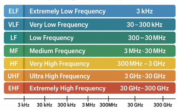
RF Bands [1]
##Structure of RF waves
RF waves are EM signals, thus in free space, or in any other homogeneous, isotropic, and non-attenuating medium, electromagnetic waves propagate as transverse waves. This means that for a plane wave, the electric field and the magnetic field are each oriented perpendicular (i.e., transverse) to the direction of propagation:
where is the wave-propagation vector.
EM Wave [2]
Antennas
Definition
An antenna is a transducer that converts electrical signals into electromagnetic waves for transmission, and vice versa for reception. It is one of the most critical components in any RF communication system, as it directly determines how effectively a signal is radiated, captured, and transferred through free space.
Principle of Operation
Antennas operate based on the physics of electromagnetic radiation. When an alternating current flows through a conductor, it creates a time-varying electric and magnetic field. If these fields detach from the conductor and propagate outward, electromagnetic radiation occurs. The efficiency and pattern of this radiation depend on the antenna’s geometry, resonant length, and the operating frequency.
1.1 Resonant Frequency:
Dipole Antenna and Resonance [3]
Antennas perform best when their physical length is proportional to the wavelength (e.g., λ/2 or λ/4). At resonance, energy transfer between the transmitter and the antenna is optimized.
1.2 Radiation Pattern:
This describes how an antenna radiates energy in space. Patterns can be omnidirectional (equal in all directions within a plane) or directional (focused in specific directions to increase gain).
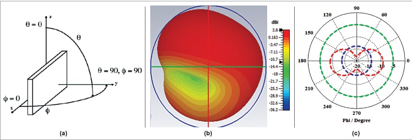
Antenna Radiation Pattern [4]
Antenna radiation patterns play pivotal role in determining choice for the IoT and Edge gateway boards.
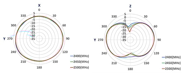
Radiation patterns graphically represent how the antenna radiates or absorbs radio energy in 3D space. Datasheets typically show the maximum extent in the XY and YZ planes when the antenna is mounted as intended. (Image source: Amphenol).
1.3 Gain:
Antenna gain measures how effectively the antenna directs power compared to an isotropic radiator. Higher gain increases the effective communication range in the direction of the main lobe. It is usually referenced to an isotropic antenna with a designation of dBi. It is calculated from the formula .
1.4 Maximum power transfer:
Efficient power transfer between an antenna and a receiver occurs when the transmission line impedance () is matched to the antenna impedance (). Poor impedance matching increases the return loss (RL). The voltage standing wave ratio (VSWR) quantifies how well the transmission line is impedance-matched to the antenna. Higher VSWR values correspond to greater power losses. For most IoT products, a VSWR below 2 is generally considered acceptable.
Antennas typically present a 50-ohm impedance. Proper matching ensures minimal reflection and maximum power transfer between the antenna and RF circuitry.
1.5 Bandwidth:
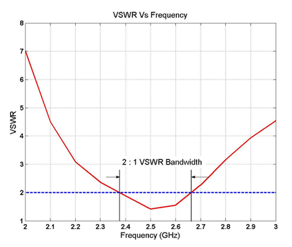
Antenna Bandwidth (Source: Mobile Mark)
The range of frequencies over which the antenna performs adequately. Wideband antennas can support multiple standards or agile frequency systems.
1.6 Polarization:
Refers to the orientation of the electric field (e.g., vertical, horizontal, circular). Matching polarization between transmitter and receiver improves signal strength.
Wireless Propagation
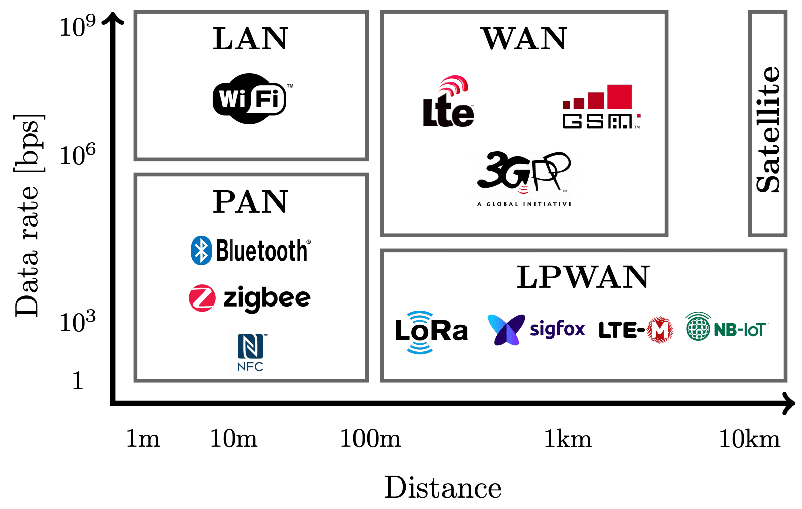
Comparison of Wireless Technologies
As shown in the Figure above, various wireless technologies provide different range and data rate. The underlying protocol stack also yields difference in energy consumption of each of these wireless technologies. For instance, LoRa provide longer range with lower data rate but good energy efficiency as compared to Bluetooth. Bluetooth is much more power-efficient then WiFi but lower data rate can be sustained. Both Bluetooth and WiFi can have comparable range. However, recent WiFi variants powered by a technology called Multiple Input Multiple Output (MIMO) provide significantly larger ranges. Some of these technologies operate in licensed spectrum, while others in Unlicensed bands. The two factors, i.e., data rate and the communication range are linked to operation frequency, and the propogation conditions. In this section, we aim to uncover the factors which characterise these two key performance measures.
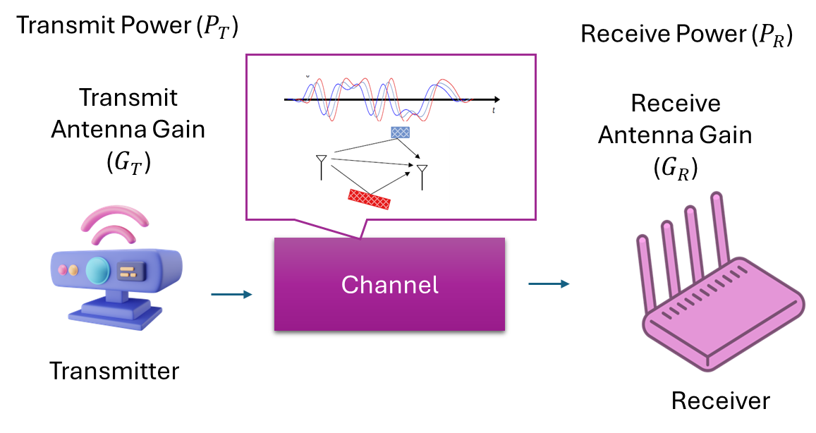
Link
Let us consider a pair of transmitter (TX) and a receiver (RX). The performance of the link formed by TX-RX pair is determined by a factor called Signal-to-Noise Ratio (SNR):
where is received Power and is the noise power on the receiver interface. Both of these are generally a random variable and you are more likely to see, average SNR as given below:
It is obvious that noise is random due to the physics of the thermal noise. The randomness in the received power comes from multiple factors:
- The received power is function of the transmit power which falls off as the distance between transmitter and reciever increases. This is known as path loss.
- The amount of power received at the receiver also depends on the gains introduced by transmit and receive antennas. For directional antennas such gain terms are function of relative alignment of antennas. However, assuming omni-directional transmission these gains are often denoted by and .
- Both of the above factors are deterministic, i.e. if we know distance between the TX-RX and may be something about how fast the power decays in some environment (again this is often random dependent on the geometric properties) then we can work out the received power. However, the scatterers present between RX and TX, may diffract, reflect or absorb RF signals. The phenomenon is known as shadowing. Shadowing is the attenuation caused by obstacles between the transmitter and receiver that absorb the transmitted signals.
- Received power variations caused by path loss occur over long distances (typically 100–1000 m), while variations due to shadowing appear over distances comparable to the size of the obstructing object (about 10–100 m in outdoor environments and even shorter indoors)Because both path-loss and shadowing effects change over relatively large spatial scales, they are collectively referred to as large-scale propagation effects.
- Beside large scale path-loss the received power varies over smaller duration due to multiple scatterers reflecting signals which can add up constructively or destructively on receiver. This is known as fading or small-scale propogation effect. Constructive and destructive interference between multipath components occurs over very short distances—on the order of the signal wavelength—because each component’s phase completes a full 360° rotation over that distance. As a result, power variations caused by multipath are referred to as small-scale propagation effects.
Propagation between TX-RX.
The Figure above shows some of the factors which we will explore in details. All the phenomenon's encountered can be seen when we plot the , figure below shows this quantity plotted on dB scale against the distance (on log scale).
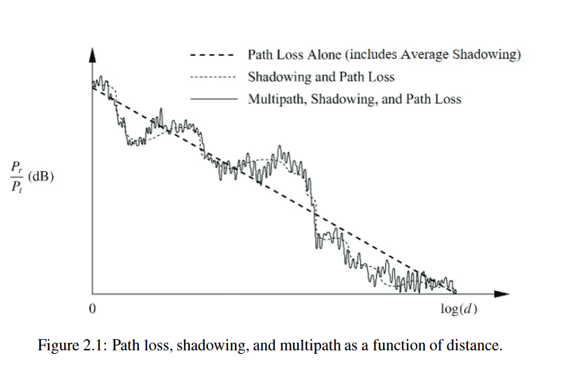
Propagation Impairments (Source: Goldsmith [5]).
Transmit Power
Transmit power refers to the amount of power a radio transmitter outputs, typically expressed in watts (W), dBW, or dBm (decibels relative to 1 milliwatt). Since transmitters rely on power amplifiers, the achievable transmit power is largely determined by amplifier design and efficiency. A useful analogy is a light bulb—a higher-wattage bulb emits more light, just as a higher-power transmitter radiates a stronger signal. Below is a table of typical approximate transmit power levels for common wireless technologies.
| Technology | Power (W) | Power (dBW) |
|---|---|---|
| Bluetooth | 10 mW | -20 dBW |
| Wi-Fi | 100 mW | -10 dBW |
| LTE Base Station | 1 W | 0 dBW |
| FM Broadcast Station | 10 kW | 40 dBW |
Path loss
Path loss is a fundamental concept in wireless communication and plays a central role in the design and performance analysis of IoT networks. It quantifies the reduction in received signal power as a function of propagation distance, frequency, antenna heights, and the physical environment. Since IoT devices are typically low cost, energy constrained, and often deployed in large numbers across diverse environments such as factories, homes, farms, and cities, accurate prediction of path loss is essential for reliable connectivity, power budgeting, and network planning.
Free-Space Path Loss
A common starting point for path loss modelling is the free space propagation model, which describes ideal line-of-sight (LoS) communication without obstructions. The received power is given by the classical Friis transmission equation
where is transmitted power, and are antenna gains, is the wavelength, and is the separation between transmitter and receiver. Rearranging this yields the free space path loss
expressed in decibels. Although this model assumes perfect line of sight conditions, it is relevant for certain Internet of Things domains such as long range low power wide area networks operating in open rural areas. If we ignore shadowing and fading for now, we can start with preliminary link budget analysis. The link budget tells us what received power we should expect, this should be above a certain threshold so that the receiver can function. We also measure received power on the receiver as Receive Signal Strength Indicator (RSSI). LoRAWAN is a Long range Wide area networking (LoRAWAN) technology, let us understand the link budget using a case-study as follows.
LoRaWAN Free-Space Path Loss Example
Path loss for LoRaWAN devices can be estimated using the free-space Friis equation:
where is the distance in meters and is the frequency in MHz.
Assume a LoRaWAN device transmitting at with 0 dBi antenna gain. The free-space path loss at different distances is calculated as follows:
1. Distance: 1 km
Received power for a 14 dBm transmitter with 0 dBi antennas:
2. Distance: 2 km
3. Distance: 5 km
These calculations demonstrate that LoRaWAN can maintain reliable links over kilometers in rural or open environments, since the received power remains well above typical receiver sensitivities around -130 dBm. Obviously these are very simple calculations which ignore quite a lot of details including the noise power which impacts the receiver performance.
Path loss Exponent
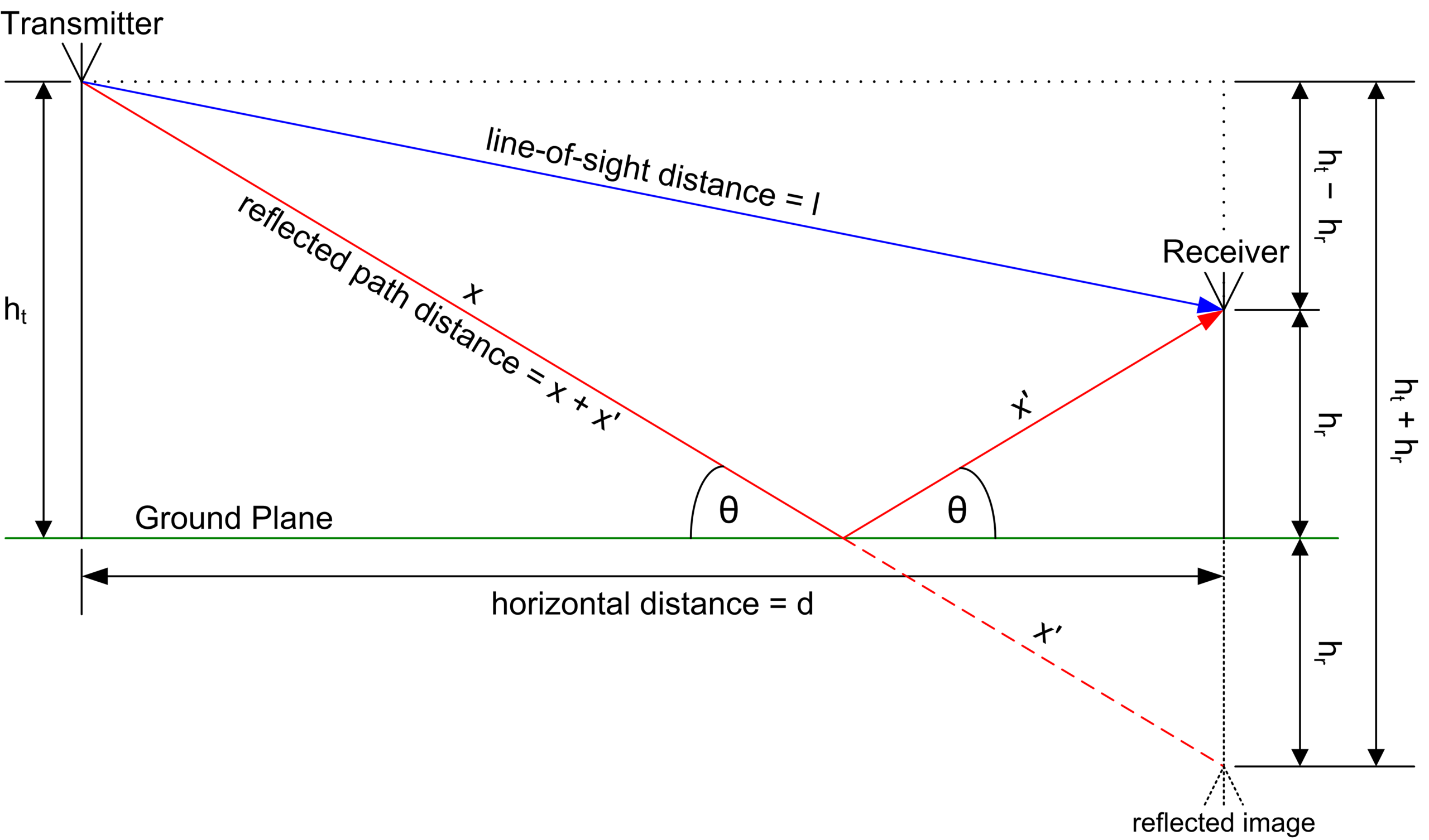
Two Ray Propagation Model (Source: Wikipedia).
How fast does the power attenuate in real world depends on the propagation environment. Unlike, free space where the power decays as inverse square-law, in reality it can go down much faster. To appreciate this consider two-ray ground model. The Two-Ray Ground Reflection model is a widely used radio propagation model that accounts for both the direct line-of-sight path and a single ground-reflected path. In this model, the total received electric field is the sum of the direct path and the ground-reflected path. Assuming the transmitted signal has power and the antennas have gains and , the received power can be expressed as:
Where:
- is the direct line-of-sight distance
- is the distance of the ground-reflected path
- is the reflection coefficient of the ground
- is the wave number
- represents system losses
For simplicity, when the distance is much greater than the antenna heights, and the antennas are approximately the same height , the received power simplifies to:
Where:
- and are the transmitter and receiver antenna heights
- is the horizontal separation between antennas
The corresponding path loss in decibels can be expressed as:
This shows that at large distances, the path loss increases with the fourth power of distance, in contrast to free-space path loss, which increases with the square of distance. This shows that merely one reflection can double the way power attenuates. So in general, we can write the path-loss as
where is some reference distance for antenna far-field and is the path-loss exponent. Some indicative values of are presented in [5], summarised as follows:
| Environment | (Path Loss Exponent) Range |
|---|---|
| Urban macrocells | 3.7–6.5 |
| Urban microcells | 2.7–3.5 |
| Office building (same floor) | 1.6–3.5 |
| Office building (multiple floors) | 2–6 |
| Store | 1.8–2.2 |
| Factory | 1.6–3.3 |
| Home | 3 |
Multi-Slope Path Loss Model
The multi-slope path loss model generalizes traditional single-slope models by assigning different path-loss exponents to distinct distance ranges, capturing the transition from near-field free-space propagation to far-field obstructed environments. Let be the transmitter-receiver separation and be the boundaries of distance regions. The path loss is expressed as a piecewise function:
Here, is the reference path loss at , and are the path-loss exponents for each segment. This model effectively captures the change in propagation behavior caused by obstacles, foliage, or urban structures, providing a more accurate representation of signal attenuation over varying distances compared to single-slope models. It is particularly useful for long-range IoT deployments, UAV-ground links, and heterogeneous urban environments, where the path-loss exponent can transition from values close to two in near free-space regions to higher values in dense cluttered regions.
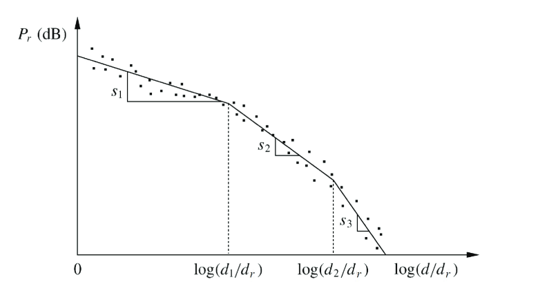
Multi-slope Path loss Model (Source: Goldsmith [5])
Shadowing
In wireless communication, a transmitted signal rarely propagates along a perfectly unobstructed path. Instead, it encounters various objects such as buildings, trees, vehicles, and other obstacles that partially or fully block the signal. These obstructions introduce random fluctuations in the received signal power at a given distance, a phenomenon commonly referred to as shadowing or slow fading. Unlike fast fading, which arises from constructive and destructive interference of multiple signal paths over small distances or short time intervals, shadowing represents longer-term variations caused by environmental features.
Shadowing occurs not only due to physical blockage but also because of changes in reflecting and scattering surfaces in the environment. For example, variations in the size, orientation, or material of nearby objects can modify how signals are reflected or scattered, further contributing to the randomness of the received power. These effects are inherently unpredictable because the precise location, dimensions, and dielectric properties of obstacles, as well as the dynamic nature of the environment, are typically unknown or difficult to measure in practice.
To capture this variability in a mathematically tractable manner, statistical models are employed. The most widely used approach represents shadowing as a log-normal random variable, reflecting the fact that received power in decibels fluctuates around its mean path-loss value according to a normal distribution. Mathematically, the received power at distance can be expressed as:
where is the mean path loss predicted by a deterministic model such as free-space or log-distance, and is a zero-mean Gaussian random variable with standard deviation that captures the effects of shadowing. This statistical characterization allows system designers to account for unpredictable environmental variations, providing more realistic predictions of link performance, coverage, and reliability in wireless networks.
Outage Probability Derivation
The outage probability is the probability that the received power falls below a required threshold :
where . Since shadowing is log-normal, the total path loss in dB is normally distributed:
Using the standard normal cumulative distribution function , the outage probability is:
This expression shows that the outage probability increases with the distance as grows, and also increases with larger shadowing standard deviation .
Case Study: LoRaWAN Link Distance under Urban Shadowing with FSPL Comparison
In urban environments, LoRaWAN devices are strongly affected by shadowing caused by buildings, vehicles, and other obstacles. This case study demonstrates how log-normal shadowing impacts link distance and compares the results to a simple Free-Space Path Loss (FSPL) prediction.
Scenario
- Deployment: LoRaWAN network in a dense urban area
- Frequency: 868 MHz
- Transmitter power: 14 dBm
- Antenna gains:
- Path-loss exponent: (urban)
- Shadowing standard deviation:
- Receiver sensitivity:
- Outage probability target: (10%)
The log-distance path-loss model with shadowing is:
where and the reference path loss at is:
Outage Probability and Link Distance
The outage probability is:
where .
Solving for the maximum distance given the outage target:
Numerical Calculation:
Comparison to FSPL Model
The Free-Space Path Loss (FSPL) model predicts the received power without considering shadowing or urban clutter:
- Solving for the distance at the same threshold :
Insight:
- FSPL overestimates coverage in urban areas because it ignores obstacles and shadowing.
- The log-normal shadowing model provides a more realistic link distance of 1.34 km for a 10% outage probability, compared to 5.9 km predicted by FSPL.
- This comparison highlights the importance of statistical modeling for urban IoT network planning.
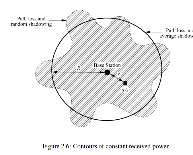
Coverage (Source: Goldsmith [5])
Essentially, the coverage is squashed in various directions by the shadowing as shown above.
Miscellaneous Losses in Wireless Communications
When designing a link budget, it's important to account for miscellaneous losses beyond the main path loss. These are typically grouped together into a single term, often in the range of 1–3 dB. Common sources of these losses include:
- Cable loss: Signal attenuation due to the transmission line connecting the transmitter or receiver to the antenna.
- Atmospheric loss: Signal absorption or scattering caused by the atmosphere, which varies with frequency and distance.
- Antenna pointing errors: Misalignment between the transmitter and receiver antennas, reducing effective received power.
- Precipitation: Rain, snow, or other weather effects that absorb or scatter radio waves.
The plot below illustrates atmospheric loss in dB/km as a function of frequency (we typically operate below 40 GHz). For short-range links under 1 km, the atmospheric loss is generally less than 1 dB, so it is often negligible. However, atmospheric loss becomes significant in satellite communications, where the signal must traverse many kilometers through the atmosphere.

Atmospheric Losses (Source: PySDR)
Multi-path Fading
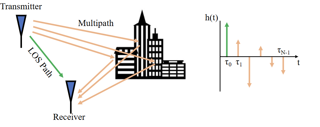
Mulitpath Propagation (Source: PySDR)
- In a real-world wireless channel, the signal you transmit doesn’t travel along a single straight line (line-of-sight), but typically many paths: reflections off buildings, ground reflections, diffraction around obstacles, scattering from rough surfaces/objects.
- Each path has a different length → different delay, and different attenuation → different amplitude. Also, different paths incur different phase shifts. At the receiver, all paths sum (superpose): they may add constructively (reinforce) or destructively (cancel). That is “multipath.”
- Because of this summation, the received signal’s amplitude and phase fluctuate over time (if Tx, Rx or environment moves) or over frequency — this phenomenon is called fading.
Types of Fading
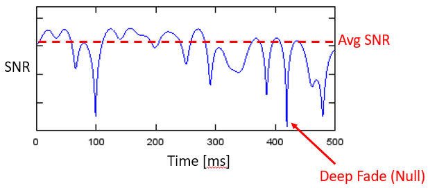
Deep Fading (Source: PySDR)
| Classification | Phenomenon | Description |
|---|---|---|
| Time domain | Slow fading vs Fast fading | Slow fading: channel roughly constant over a packet; a deep fade may wipe out entire packet. Fast fading: channel changes quickly (within or across symbols), causing rapid SNR fluctuations. |
| Frequency domain | Flat fading vs Frequency-selective fading | Flat fading: signal bandwidth is narrow compared to channel coherence bandwidth → all frequencies experience similar attenuation/phase. Frequency-selective: wideband signal spans many wavelengths → different frequency components undergo different fading, possibly causing some frequencies to be deeply faded while others are not. |
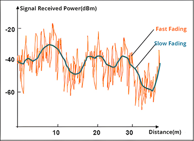
Fast vs Slow Fading (Source: PySDR)
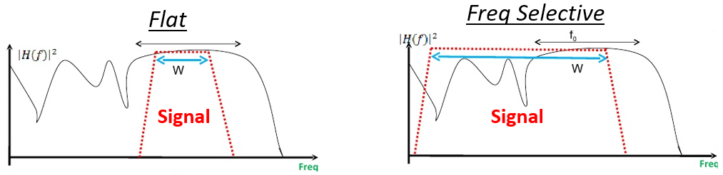
Flat and Frequency Selective (Source: PySDR)
Additional notes:
- Delay spread: signals from different paths arrive at different times → can cause inter-symbol interference (ISI).
- Doppler / mobility effects: movement causes channel response to vary over time (time selectivity) → fading + Doppler spread.
Statistical Channel Models
Because the exact multipath geometry is usually unknown and constantly changing, it's common to model the channel statistically:
- Rayleigh fading: No dominant line-of-sight (LOS) path; envelope of received signal follows a Rayleigh distribution.
- Rician fading: Dominant LOS path + scattered multipath; envelope follows a Rician distribution.
More advanced models include composite fading and clustering of paths, but Rayleigh and Rician are classical.
Mathematical / Signal-Processing View
From a system perspective, the multipath channel can be modeled as a linear time-varying filter:
-
Each path has delay and complex gain .
-
Flat fading: all paths experience roughly the same amplitude/phase.
-
Frequency-selective fading: delays spread across symbols → multi-tap channel.
-
Statistical models treat , as random variables/processes.
Mitigation Techniques
- Diversity: multiple antennas, frequency hopping, or time interleaving.
- Channel coding + interleaving: combats deep fades affecting short symbol bursts.
- Equalization: compensates for delayed multipath (reduces ISI).
- Multicarrier modulation (OFDM): splits wideband channel into flat subcarriers.
- Adaptive modulation / power control: adjust transmit parameters based on channel quality.
Signal Spreading to Counter the Fading
One effective way to mitigate multipath fading is to spread the signal across time or frequency, making it more resilient to deep fades in any one narrow band. This is the principle which allowed 3G wireless networks to operate based on code division multiplexing (CDMA). The coding technique spreads the transmission over wider bandwidth allowing better immunity.
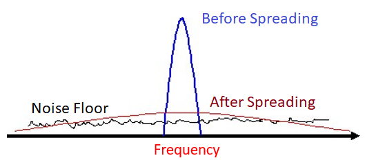
CDMA (Source: PySDR)
Intuition: Why Spreading Helps
- In a flat-fading channel, the received signal can experience rapid amplitude fluctuations due to constructive and destructive interference from multipath.
- If the transmitted signal occupies a very narrow band, a deep fade can wipe out the entire signal.
- By spreading the signal over a wider bandwidth or longer duration, different parts of the signal experience different channel conditions.
- Some portions may fade less or not at all.
- At the receiver, combining all the portions averages out the fades → higher probability of correct reception.
Mathematically, if a narrowband signal (s(t)) is multiplied by a spreading code (c(t)) or chirp, the received energy is distributed over multiple fading realizations, reducing variance of the received amplitude.
Chirp Spread Spectrum (CSS) & LoRa
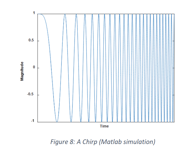
Chirp (Source: LoraWAN Semtech)
Chirp Spread Spectrum (CSS), used in LoRa, is a practical implementation of this principle:
- A chirp sweeps the signal linearly across a wide bandwidth.
- The spreading factor (SF) controls how long the chirp lasts (time-domain spreading):
- Higher SF → longer chirps → more spreading → better immunity to fading and noise.
- Trade-off: higher SF reduces data rate but improves link reliability.
Why CSS/LoRa works particularly well against fading:
- Time-Frequency Diversity: A single deep fade in frequency only affects a small part of the chirp; the rest still conveys information.
- Processing Gain: Longer spreading (higher SF) allows the receiver to integrate energy over a long chirp, boosting SNR and effectively “averaging out” fades.
- Resistance to Multipath: Chirps are wideband signals; even in a frequency-selective channel, the energy at multiple frequencies ensures at least partial recovery.
- Simplified Demodulation: CSS uses correlation with the transmitted chirp pattern; fades that affect only part of the chirp do not prevent detection.
In practice, LoRa devices often use SF between 7 and 12: higher SF is chosen for longer-range or harsh multipath environments because it maximizes spreading and resilience to fading. We will cover the specific modulation aspects in details later.
Orthogonal Frequency Division Multiplexing (OFDM)
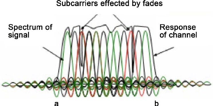
OFDM (Source: Research Gate)
Orthogonal Frequency-Division Multiplexing (OFDM) combats frequency-selective fading by splitting a wideband signal into many narrowband subcarriers, each carrying a portion of the data. Because each subcarrier has a bandwidth much smaller than the channel's coherence bandwidth, it experiences approximately flat fading, even if the overall channel is highly frequency-selective. This simplifies equalization, as the receiver only needs to correct a single complex gain per subcarrier rather than a full multi-tap channel. By converting a difficult frequency-selective channel into a set of independent flat-fading subchannels, OFDM makes reliable high-speed communication possible in multipath-rich environments.
Overall Channel Gain
Assuming that the channel is frequency flat, and is single tap allows us to simplify the calculation of the overall received power as
- = transmitted power
- = antenna gains
- = reference distance
- = link distance
- = path-loss exponent
Outage Probability with Rayleigh Fading and Lognormal Shadowing
Outage probability is the probability that the received power falls below a threshold :
Using the composite fading model:
Let us define the deterministic received power (path loss only):
Then:
The outage condition becomes:
Let:
The composite fading variable is the product of a Rayleigh and a lognormal random variable. The outage probability is:
Where:
- is the CDF of Rayleigh fading ()
- is the PDF of lognormal shadowing:
So:
The outage probability for a composite lognormal shadowing + Rayleigh fading channel is:
If we ignore lognormal shadowing (), the received power reduces to:
The outage condition becomes:
For Rayleigh fading, has CDF:
Thus, the outage probability with Rayleigh fading only is:
Where:
- is the mean power of the Rayleigh fading envelope
This is the classical Rayleigh-only outage probability, which is widely used for simple link-budget calculations when shadowing is negligible.
Noise
So far we have ignored the noise on the receiver front-end. We want to compare the energy contribution from our signal to the energy contribution from noise. To quantify the noise contribution, we calculate the noise spectral density, which represents the noise power per unit of bandwidth. In most cases, the dominant source of noise is thermal noise. The thermal noise spectral density is given by:
where:
- is the Boltzmann constant (Joules per Kelvin),
- is the system noise temperature (Kelvin),
- is the total noise power (Watts), and
- is the bandwidth (Hertz).
This relationship allows us to relate the noise power over a given bandwidth to the fundamental thermal noise present in the system.
System Noise Temperature
The total input noise temperature of a system, , has contributions from both the antenna and the receiver:
- is the antenna noise temperature, representing the noise power seen at the output of the antenna. This is primarily thermal in nature and depends on the observing frequency and what the antenna is pointed at (for example, cold space vs. the hot Earth).
- is the receiver noise temperature, representing noise generated by the internal components of the receiver.
Receiver Noise Temperature and Noise Factor
The receiver noise temperature is usually expressed in terms of a noise factor , which quantifies the increase in noise power referred to the input of a component or system, assuming a reference input noise temperature :
The noise factor is defined as:
It is common to express the noise factor in decibels, called the noise figure :
Interpretation: The noise figure represents the reduction in signal-to-noise ratio (SNR) caused by passing a signal through a system, assuming the source has a noise temperature of 290 K.
Example: If an amplifier has K, then its noise figure is dB. When amplifying a source at room temperature ( K), the amplifier insertion reduces the SNR by 6 dB.
Total System Noise Temperature
Combining the antenna and receiver contributions:
The thermal noise power can be approximated using:
where:
- is the system bandwidth in Hz
- is the receiver noise figure in dB
- is the thermal noise floor at room temperature
LoRaWAN Receiver Sensitivity Calculation
The thermal noise floor for a receiver can be estimated as:
For a bandwidth of :
Adding the receiver noise figure (NF) and the required minimum SNR, the receiver sensitivity is:
Many LoRa modules report similar or even better sensitivities in practice, depending on the spreading factor and implementation. The table below summarises the key values.
| Parameter | Value (typical / assumed) |
|---|---|
| Thermal noise floor (room temp) | –174 dBm/Hz |
| Receiver Noise Figure (NF) | ~ 6 dB |
| Receiver equivalent noise temperature Tn | ≈ 870 K (for NF = 6 dB) |
| Bandwidth examples | 125 kHz (common for LoRa), 200 kHz (NB‑IoT), etc. |
| Resulting noise floor (125 kHz BW) | –174 + 10 log₁₀(1.25e5) ≈ –123 dBm |
| Sensitivity (typical LoRa, SNRmin = –20 dB) | –124 + 6 – 20 ≈ –138 dBm |
| Sensitivity (less aggressive, e.g. NB‑IoT 200 kHz, SNR ≈ –1 dB) | –174 + 10 log₁₀(2e5) ≈ –117 dBm → –117 + 6 – 1 ≈ –112 dBm |
Signal-to-Noise-Ratio
Putting all of this together, we can now write SNR as
where and . The outage probability in terms of SNR is then defined as:
Shannon Capacity and SNR Relationship
The Shannon capacity defines the theoretical maximum data rate that can be achieved over a communication channel without error, given its bandwidth and signal-to-noise ratio (SNR). For a channel with bandwidth and received SNR (linear scale), the capacity in bits per second is given by the Shannon-Hartley theorem:
Here, the SNR is defined as:
where is the received signal power and is the total noise power, including thermal noise and the receiver noise figure. The logarithmic relationship shows that capacity increases with SNR, but with diminishing returns: doubling the SNR does not double the capacity.
In practical wireless systems, the SNR is influenced by path loss, shadowing, fading, interference, and receiver noise figure, making Shannon capacity a theoretical upper bound rather than a guaranteed rate. Nevertheless, it provides a fundamental benchmark for designing and evaluating IoT, LoRaWAN, and UAV communication links, guiding modulation, coding, and power allocation strategies to approach the channel's maximum achievable throughput.
References
[1] IC-Component's Blog, "What Is Radio Frequency (RF) Technology? Structure, Uses, and Signal Behavior", July, 2025.
[2] Wikipedia, "Polirization of Waves", accessed on December 2025.
[3] Dinobell, "Antenna Resonance", 2025
[4] S. Shungati, "The Importance Of Radiation Pattern Of An Antenna", Electronics Forum, 2024.
[5] Goldsmith, Andrea. Wireless communications. Cambridge university press, 2005.
[6] Shooshtary, Samaneh. Development of a MATLAB Simulation Environment for Vehicle-to-Vehicle and Infrastructure Communication Based on IEEE 802.11p.