
Lecture 3 - Part 1
Contents
- Introduction
- Probability Theory
- References
Introduction
Probability Theory
Before introducing the detection, estimation, and forecasting techniques in details, it is important to understand some key probabilistic concepts. The probability theory itself merits an entire course on its own. Therefore, it is challenging to cover all aspects as part of one chapter. Interested readers are referred to [1] for the detailed exposition of the topic.
Sample Space
Let us consider an experiment, e.g., tossing of a coin or dice, predicting the location of a ball in roulette etc. The outcome of such experiment is random and not predictable with certainty. Nevertheless, we do know that tossing a coin will result in head/tails, or in case of dice it will result in a number between 1-6. Consequently, while the outcome of the experiment is not known and its random, the set of all possible outcome is known.
Definition
The set of all possible outcomes of an experiment is known as the Sample Space and is commonly denoted by .
Examples
- Coin Toss: In case of coin-toss example, , i.e. the outcome is either heads() or tails().
- Student Exam: Consider a cohort of five students appearing in exam. Then the outcome is the position of the student after the test, i.e.
the outcome (2,3,4,1,5) for instance means that the student with ID 2 came first in the test and so on.
- Double Coin-toss: In case of flipping two coins, the sample space can be defined as all possible combinations as:
One can appreciate from this example that the is a product space of the sample space of single coin-tosses .
Event
Definition
Any subset of sample space is known as event. In other words, an event () is a set of possible outcomes for the experiment.
If the outcome of the experiment is contained in set E, we say that event E has occurred. For instance, consider following examples:
- Rolling a dice: Consider rolling a dice, then an event can be rolling an even number, i.e.
- Double coin-toss: Imagine flipping two coins, then an event can be that at least one tail appears, i.e.,
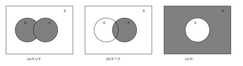
Let and be two events in then will occur when either or occurs. The event is called a union event. Similarly, we can define an event which is an intersection of and , i.e., contains all outcomes which are feasible when both and occur. If is then and are mutually exclusive events. The set is complementary set of often denoted by or . Generally, the unions and intersections of the events can be defined as:
Some examples of these three concepts are as follows:
Example 1: Rolling a Die
The sample space is
Let
- (event that the outcome is even),
- (event that the outcome is at least 4).
Then:
- Intersection:
is the event that the outcome is even and at least 4.
- Union:
is the event that the outcome is even or at least 4 (or both).
- Complement:
is the event that the outcome is odd.
Example 2: Drawing a Card
The sample space is
Let
- (13 cards),
- (12 cards).
Then:
- Intersection:
is the event that the card is a heart and a face card.
- Union:
is the event that the card is a heart or a face card (or both).
- Complement:
is the event that the card is not a face card.
Algebra of Events
The operations of forming unions, intersections, and complements of events obey certain rules similar to the rules of algebra.
We list a few of these important laws:
Commutative Laws
Associative Laws
Distributive Laws
De Morgan's Laws in Probability
For two events and :
- Union complement:
- Intersection complement:
Explanation:
- contains all outcomes not in or .
- contains all outcomes not in both and .
Axioms of Probability
Probability can be defined in number of ways. One way of defining the probability is in terms of relative occurrence of the event:
where is probability of the event, is the number of times the event occurs in runs of the experiment. In other words, is defined as the limiting proportion of time that occurs. It is thus a limiting frequency of . This can be verified by a small demo here.
Dice Roller
Law of Large Numbers
Suppose we roll a fair six-sided die. The theoretical probability of getting a is .
If we perform rolls and observe outcomes equal to 3, then the empirical probability is
As , converges to .
Notice, that the definition here inherently assumes that the converges to a finite value for all repetitions of the experiment. It is difficult to prove this without making assumption on the convergence. Therefore, modern probability theory rather adopts an axiom based approach. In particular, for each event , we assume that is the probability of the event which satisfies the following axioms:
Axiom 1
The probability of an event takes value between 0 and 1.
Axiom 2
The outcome of an experiment is a point in with probability 1.
Axiom 3
For any sequence of events which are mutually exclusive, i.e., when , then
If events are mutually exclusive, then the chance of at least one happening is just the total of their separate chances.
Key Propositions in Probability Theory
1. Probability of the empty set
Statement:
Proof:
The empty set is disjoint from and . By additivity,
Subtract from both sides and use :
2. Boundedness
Statement:
Proof:
Non-negativity gives . Also , and with and disjoint, so by additivity
since . Hence . Combining yields .
Experiment: Toss a fair coin.
- Sample space:
- Event:
Probability:
3. Complement Rule
Statement:
Proof:
Because and are disjoint and ,
Rearrange to get .
Experiment: Roll a fair die.
- Event (even)
- Complement (odd)
Probabilities:
Check complement rule:
4. Sub-additivity (union bound)
Statement:
Proof:
Start from the inclusion–exclusion identity (proved below):
Since , subtracting it makes the right-hand side .
Experiment: Draw a card from a deck of 52.
- Event : heart ()
- Event : king ()
Intersection:
Union bound:
Actual probability:
5. Difference Rule
Statement:
Proof:
Partition into disjoint sets and :
By additivity,
Rearrange to obtain the stated identity.
Experiment: Roll a die.
- Event
- Event
Then
Probabilities:
Check difference rule:
6. Inclusion–Exclusion (two events)
Statement:
Proof:
Write as a disjoint union:
with the three pieces pairwise disjoint. By additivity,
But
Adding these and subtracting yields
Experiment: Draw a card from a deck of 52.
- Event : heart ()
- Event : king ()
- Intersection: king of hearts ()
Check formula:
7. Inclusion–Exclusion (general form)
Statement:
For events ,
Proof (sketch by induction):
Base is trivial. For we have the two-event formula. Assume it holds for events. Let
. Then
Apply the induction hypothesis to . Note that
so apply inclusion–exclusion again inside. Collecting terms produces the alternating sum for sets.
Experiment: Roll a die.
Intersections:
Formula:
Substitute values:
8. Monotonicity
Statement:
If then
Proof:
When , we can write . By additivity,
Since , it follows that .
Experiment: Roll a die.
Since :
Conditional Probability
Suppose that we draw one card from a standard deck of 52 playing cards, and suppose that each of the 52 possible outcomes is equally likely to occur and hence has probability
Suppose further that we are told that the card drawn is a heart. Then, given this information, what is the probability that the card is a face card (Jack, Queen, or King)?
To calculate this probability, we reason as follows: Given that the card is a heart, there can be at most 13 possible outcomes of our experiment, namely,
.
Since each of these outcomes originally had the same probability of occurring, the outcomes should still have equal probabilities. That is, given that the card is a heart, the (conditional) probability of each of the outcomes is
whereas the (conditional) probability of the other 39 points in the sample space is 0.
Hence, the desired probability will be
since there are 3 favorable outcomes: .
If we let and denote, respectively, the event that the card is a face card and the event that the card is a heart, then the probability just obtained is called the conditional probability that occurs given that has occurred and is denoted by
Definition
A general formula for that is valid for all events and is derived in the same manner: If the event occurs, then, in > order for to occur, it is necessary that the actual occurrence be a point both in and in ; that is, it must be in . Now, > since we know that has occurred, it follows that becomes our new, or reduced, sample space; hence, the probability that the event occurs will equal the probability of relative to the probability of . That is, we have the following definition:
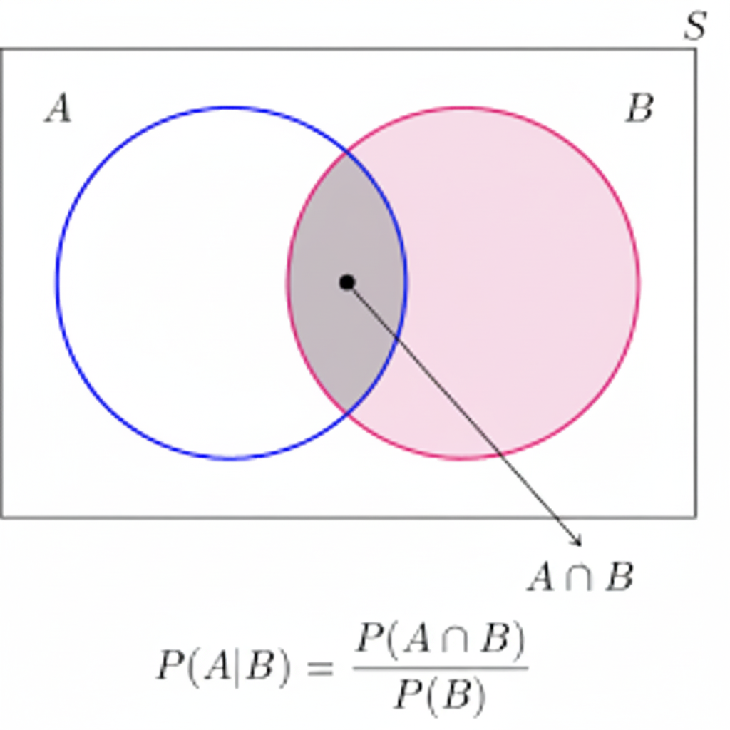
Figure 2: Visual representation
Multiplication Rule in Probability
The multiplication rule expresses the probability of the intersection of events in terms of conditional probabilities. For events , the joint probability can be written as:
Or using product notation:
Bayes Theorem
Bayes' Theorem provides a systematic way to update the probability of an event when new evidence is observed.
It is based on the idea that the posterior probability depends on:
- The prior probability , representing our initial belief before seeing the evidence,
- The likelihood , the probability of observing the evidence if the event occurs, and
- The total probability of the evidence , which normalizes the posterior to ensure all probabilities sum to 1.
Definition
Formally, Bayes' Theorem is:
If the evidence can occur under a set of mutually exclusive and exhaustive events , then the Law of Total > Probability gives:
Combining these gives the full form of Bayes’ Theorem:
This formula shows that the posterior probability increases if the evidence is more likely when occurs (higher likelihood) or if > the prior probability is larger, but it is moderated by how likely the evidence is overall.
Example 1: Low prevalence, high test accuracy.
Consider a medical test for a rare condition:
- = "person has the condition" with ,
- = "person does not have the condition" with ,
- (sensitivity),
- (false positive rate).
Then the probability of having the condition given a positive test is:
Even though the test is positive, the posterior probability rises only to 16%, because the condition is rare and false positives are possible.
Counterexample: Higher prevalence, lower test accuracy.
Now suppose the condition is more common and the test is less accurate:
- ,
- ,
- ,
- .
Then the posterior probability is:
A positive test now increases the probability from 30% to 60%, showing how higher prevalence and lower accuracy can still produce a strong posterior probability.
Key Takeaways:
- Bayes’ Theorem combines prior knowledge and new evidence to produce a rational update of probabilities.
- The denominator (total probability of the evidence) ensures the posterior is properly normalized.
- Posterior probabilities depend on prevalence, likelihood, and false positive/negative rates.
- It provides a quantitative framework for reasoning under uncertainty, widely used in many fields.
Practical Applications of Bayes’ Theorem
General Applications:
- Medical Diagnosis: Estimating the probability of disease given test results, as shown above.
- Risk Assessment: Calculating likelihoods of rare events (e.g., accidents, system failures).
- Decision Making: Updating beliefs based on new evidence in finance, law, and engineering.
- Fault Detection: In manufacturing or electronics, estimating the probability of failure given observed signals.
- Spam Detection: Filtering emails based on the probability that certain words indicate spam.
Some usage examples are as follows:
1. Spam Email Classification (Naive Bayes)
Suppose we want to classify an email as spam () or not spam () based on the presence of the word "discount" ().
- Prior probability: ,
- Likelihoods: ,
Compute the probability that the email is spam given it contains "discount":
Interpretation: The email is approximately 63.6% likely to be spam given it contains the word "discount".
2. Disease Prediction in ML Model (Binary Classification)
Suppose a binary classifier predicts a disease based on a symptom feature:
- Prior probability: ,
- Likelihoods: ,
Compute the posterior probability:
Interpretation: Even though the symptom is strongly associated with the disease, the posterior probability is only 32.1% due to the low prevalence.
3. Feature-Based Classification in Naive Bayes
Suppose a classifier uses two independent features and :
- Prior: ,
- Likelihoods: ,
- Likelihoods for Class 0: ,
If we observe and , the posterior is:
Interpretation: Given both features are present, there is an 86.2% chance that the sample belongs to Class 1.
Example: IoT Sensor Fault Detection Using MTBF
Suppose we have a temperature sensor with a Mean Time Between Failures (MTBF) of 1000 hours. We want to determine the probability that the sensor has failed given that it shows an abnormal reading () after 200 hours of operation.
Step 1: Convert MTBF to failure probability
The failure rate per hour is approximately:
After hours, the prior probability of failure (assuming exponential distribution) is:
So, .
Step 2: Sensor behavior (likelihoods)
- If the sensor is faulty, probability of abnormal reading:
- If the sensor is working, probability of false alarm:
Step 3: Apply Bayes’ Theorem
Substitute values:
Interpretation: Given an abnormal reading after 200 hours of operation, there is approximately an 80% chance that the sensor has failed.
Insight: By combining MTBF-based prior probability and observed evidence, Bayes’ Theorem helps in predictive maintenance to identify likely sensor failures early and reduce system downtime.
Random Variable
Generally, when an experiment is performed, we are interested in functions of the outcome rather than outcome itself. For instance, we are interested in tossing two dice, if the sum of the faces adds up to 6 and not that much concerned about individual face values for each flip. Essentially, two flips can yield any of the combinations in set [(1,5), (2,4), (3,3), (4,2), (5,1)]. These functions which map the outcomes in the sample space to real value are known as Random variables. Formally,
Definition
A random variable (RV) is a function mapping outcomes to real values:
Discrete RV takes countable values (in ) while the continuous RV can take values in .
Probability Mass Function (PMF)
For a discrete random variable:
with
Example
Suppose that our experiment consists of tossing 3 fair coins. If we let denote the number of heads that appear, then is a random variable taking on one of the values and with respective probabilities
Probability Density Function (PDF)
We say that is a continuous random variable if there exists with
so that we can define the probability of some set to be
In other words, probability of RV taking some value is given by:
Cumulative Distribution Function (CDF)
For both discrete and continuous cases:
4. Expectation and Variance
Expectation (Mean):
Variance:
Inequalities of Expected Value
Expected value inequalities provide upper bounds on the probability of a random variable's value deviating from its expected value. They are used when the exact probability distribution is unknown, offering a way to make probabilistic statements with limited information.
1. Markov's Inequality
Markov's inequality is a fundamental tool that applies to any non-negative random variable. It gives an upper bound on the probability that the random variable is greater than or equal to some positive constant.
Statement: For a non-negative random variable and a positive constant , the inequality is:
Analogy: If you know the average length of a movie is 120 minutes (), you can use this inequality to say that the probability of randomly picking a movie that is 240 minutes long or longer is no more than .
2. Chebyshev's Inequality
Chebyshev's inequality is a more powerful version of Markov's that uses the variance of the random variable. It provides a tighter bound on the probability that a random variable deviates from its mean by more than a certain amount. It applies to any random variable with a finite mean and variance.
Statement: For a random variable with finite expected value and finite non-zero variance , the inequality is:
Analogy: If you're measuring the height of students and you know the average height is 5'9" with a standard deviation of 2 inches, Chebyshev's inequality guarantees that no more than of the students are either shorter than 5'5" or taller than 6'1" (i.e., more than 2 standard deviations from the mean).
3. Jensen's Inequality
Jensen's inequality is different from the others as it doesn't directly bound probabilities. Instead, it relates the expected value of a convex or concave function to the function of the expected value. It's a foundational concept in optimization and information theory.
Statement: For a convex function :
For a concave function :
Analogy: Imagine a game where your winnings are a convex function of your dice roll. Jensen's inequality tells you that your average winnings will be greater than or equal to what you'd win if the die always landed on its average value (3.5). This shows that variability can be beneficial for convex functions.
References
[1] Ross, "Signal Processing for Communications", EPFL Press, 2008.