
Lecture 1 - Part 2
Contents
- Introduction
- Sensor Signal processing
- Sensor signals
- Signal Types
- Analog Signals and Noise
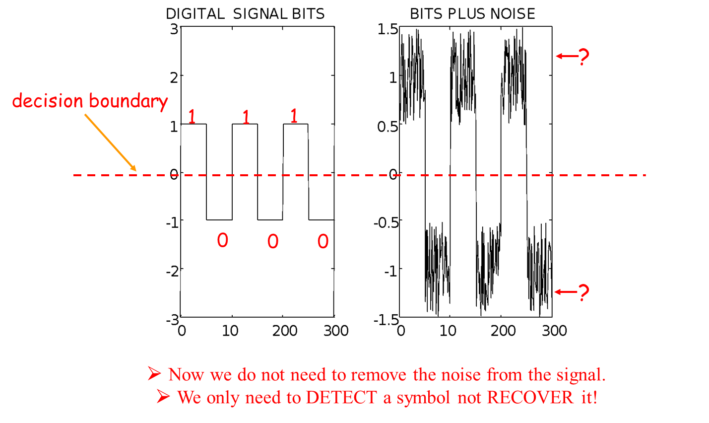
- Digital Signals and Noise
- A/D Conversion
- Sampling
- Approximating Dirac with a Real Pulse
- Fourier Series
- Fourier Transform
- Fourier Transform Pairs
- Sampling
- Nyquist Theorem
- Fourier Transform of the Impulse Train
- Fourier Transform of the Sampled Signal — Convolution in Frequency
- Interpretation — Aliasing and Nyquist
- Short Summary
- Natural Sampling
- Aliasing
Introduction
Deep-Edge Demo
Score:0
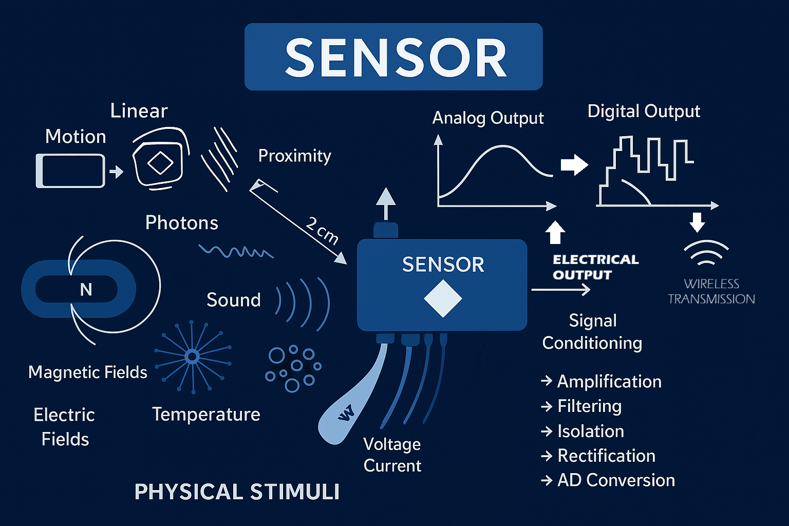
Fig 1: Sensors (Inspired by Scherz, P., & Monk, S. (2016). Practical electronics for inventors (4th ed.). McGraw-Hill Education)
Sensor Signal Processing Concepts
Select a sensor to analyze its signal conditioning and A/D conversion
Sensors
Temperature
Detect Temperature Change
Microphone
Detect sound
Photodiode
Detect variation in ambient light
Accelerometer
detect acceleration
Magnetometer
Detect changes in Magnetic Field
Flow Sensor
Detect changes in air or water flow
Signal Conditioning
Signal Conditioning
Analog-to-Digital Conversion
Samples: 0
Resolution: 256 levels
Sensor Signal processing
- Sensors are electronic or electro-mechanical components that allow devices to measure the operational environment and detect changes of physical stimuli (human/animal/nature generated).
- The sensors range from simple resistors to complex light detection and ranging (LIDARs).
- Many sensors will provide an output signal that is simply a voltage/current proportional to the property being measured.
- Some sensors use electro-mechanical structure to translate mechanical changes into electrical signals.
- Sensors provide stream of data for the Edge devices to make decisions and understand the environment.
- Sensor data is often then processed and transmitted over wireless medium.
- Several sensors may be deployed to monitor points/patterns-of-interest (PoI).
- Together these sensors form wireless sensor networks.
- Not all sensors need to be connected to Internet. Therefore, there is slight blury line between sensor networks and IoT in a strict sense.
- Sensors which have Internet connectivity can exploit secondary stream of data to understand environment better.
Sensor signals
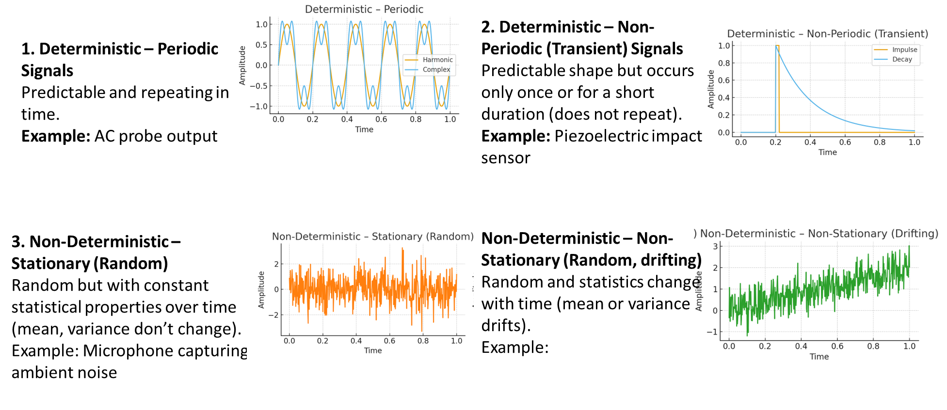
Signal Characteristics
Signal Types
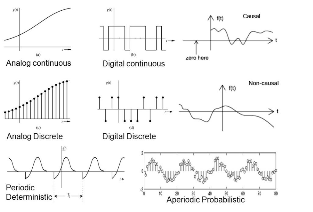
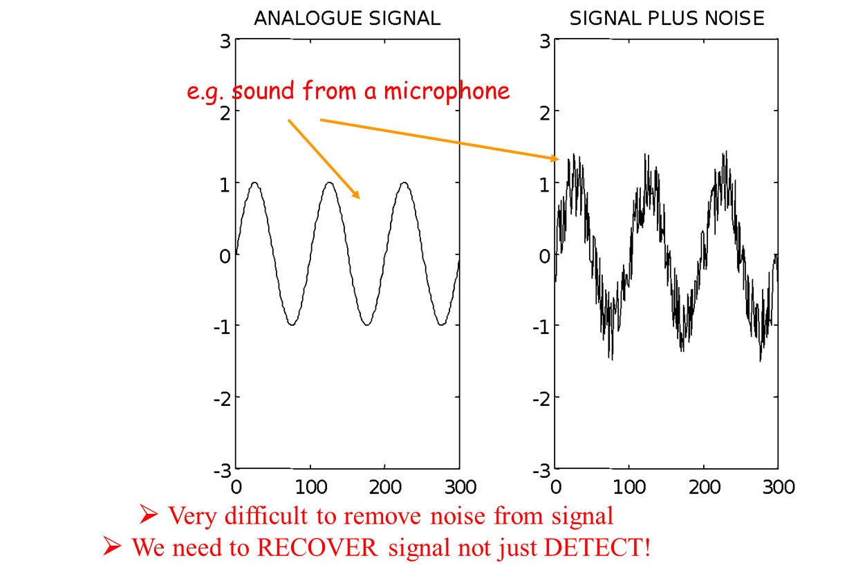
Analog Signals and Noise
Digital Signals and Noise
A/D Conversion
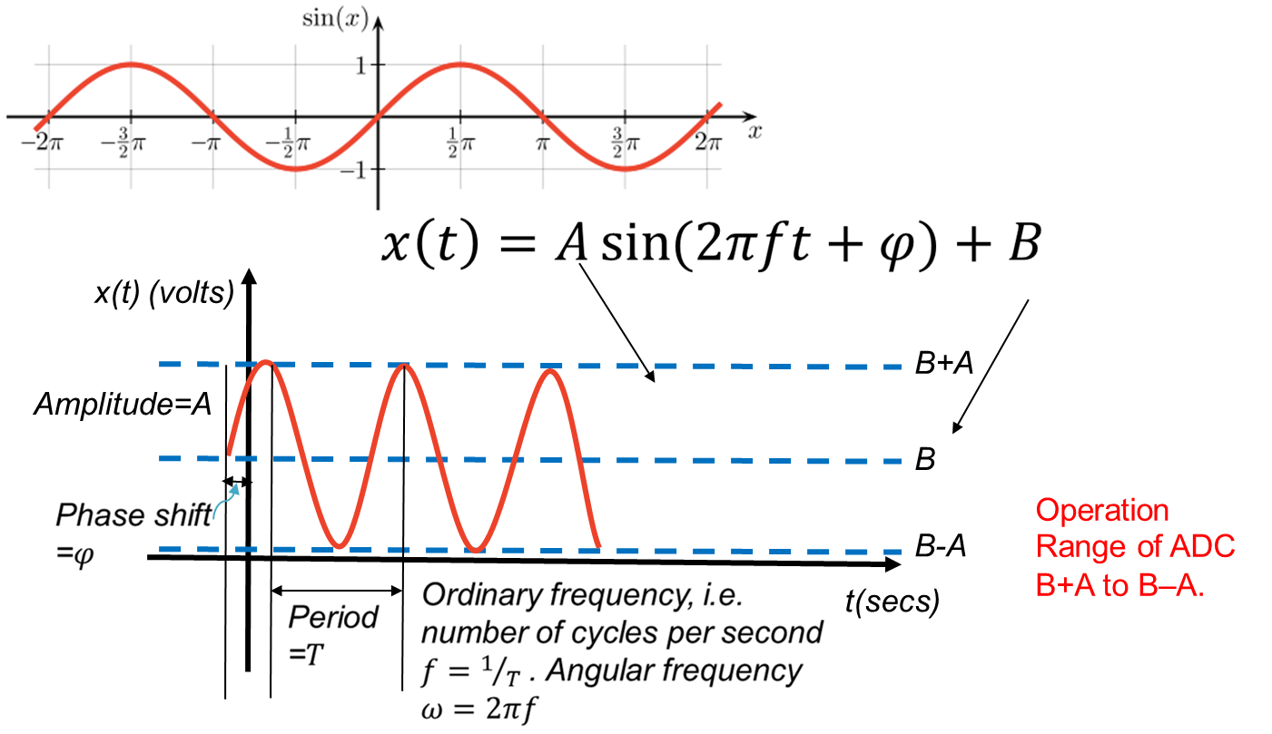
Given better noise resilience, and requirement to perform processing on the signal, we need to convert analog signals to digital. Before, we dive into sampling theory. Let us quickly recall what are the attributes of basic sine/cosine signals. We will then build our understanding of sampling in terms of these primitive signals. Later on, we will explore generalisation of these concepts.
Sampling
In order, to understand sampling process let us first understand a very important theoretical signal called dirac delta function.
Dirac Delta Function
The Dirac delta function, often denoted as , is a fundamental concept in signal processing. It is not a conventional function but a a singularity function with the following defintion:
Definition
The Dirac delta satisfies:
with the property:
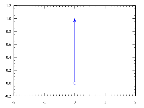
Fig 2: Dirac Delta Function
Key Properties
1.Sifting Property
This property allows the delta function to “pick out” the value of a function at a specific point.
2.Scaling Property Because the amplitude of an impulse is infinite, it does not make sense to describe a scaled impulse by its amplitude. Instead, the strength of a scaled impulse by its area.
3.Even Function
4.Shift Property
5.Multiplication by a Function
Approximating Dirac with a Real Pulse
A Dirac delta can be approximated by a real, narrow pulse of width and height , such that its area is 1:
As , in the sense of distributions.
This is useful in practice because real systems cannot generate an ideal Dirac impulse—they produce very short pulses with finite amplitude, which act like delta functions in analysis.
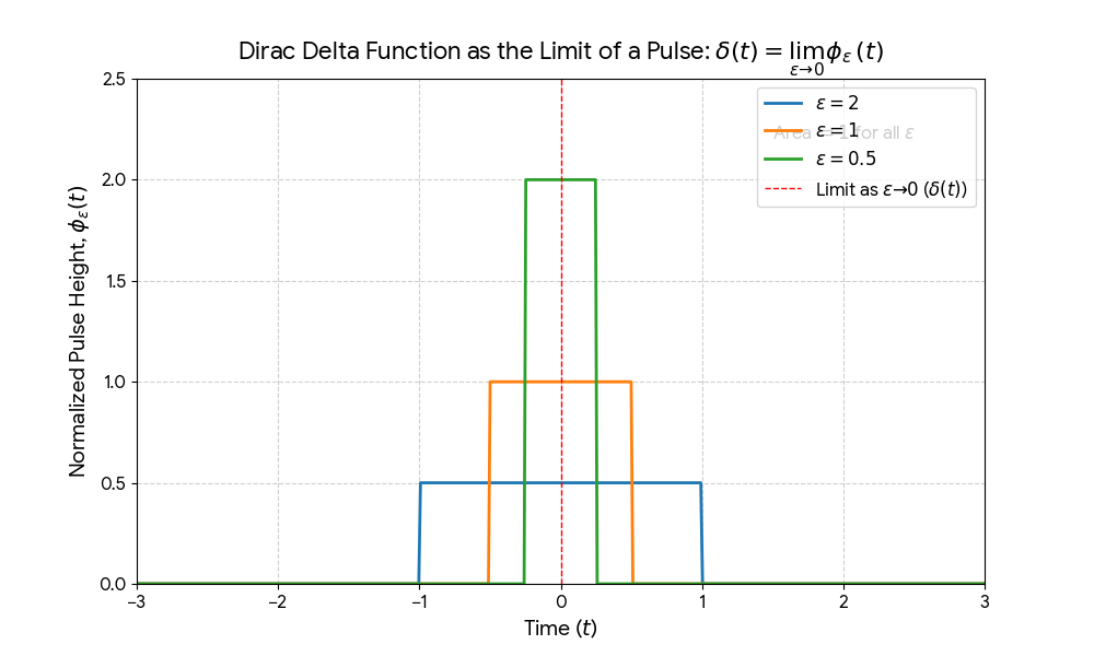
Fig 3: Impulse Approximation
The Dirac delta function can be used to describe an impulse train, i.e. collection of dirac-delta impulses as:
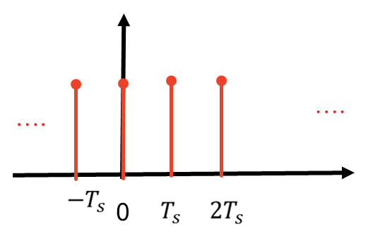
Fig 4: Impulse A continuous-time signal can be sampled as:
where is the sampling period. Employing the sifting property:
This expresses the sampled signal as a weighted sum of impulses, where the weights are the sampled values of .
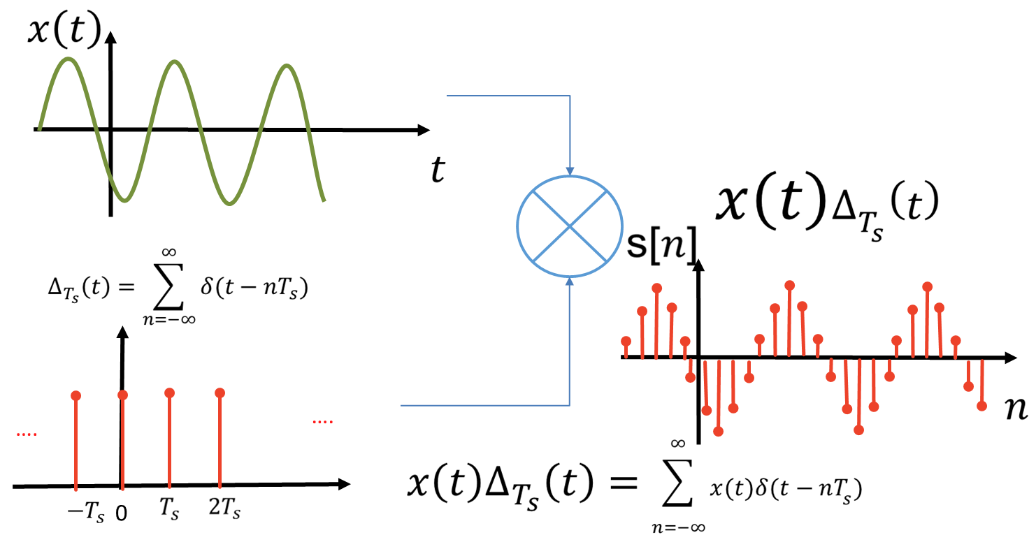
Fig 5: Sampling
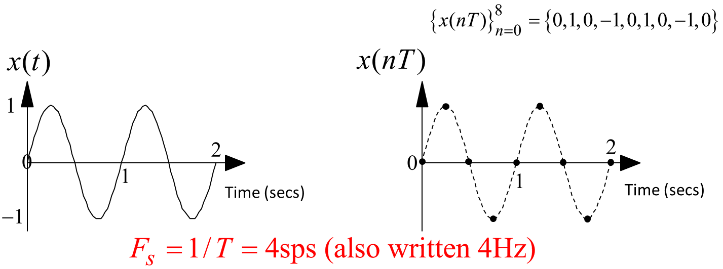
Fig 6: Sampling
Note
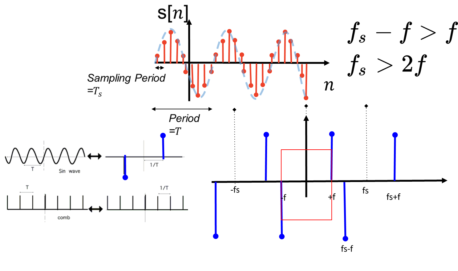
Take any analogue signal – we have used a sine wave simply as a example above. The simple question is – how fast must we sample > with an ADC so that if we transmit only the discrete-time samples (i.e. ), then > at the receiver, we can reconstruct exactly the continuous-time/analogue (with no error) by using a DAC?
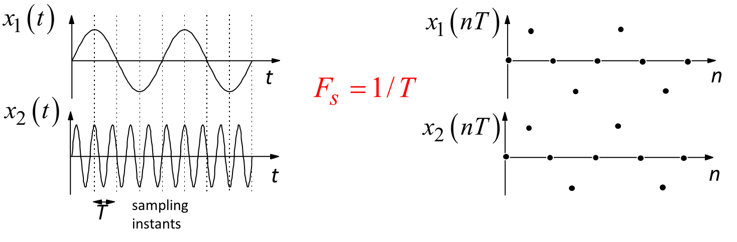
Fig 7: Sampling
Note
Clearly we have two sinusoids whose samples are identical and so the ADC will not be able to distinguish one from the other. How fast we should sample so that we can exactly reconstruct any analogue signal from its samples.
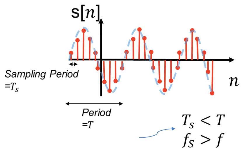
Fig 8: Some Insight
The figure above clearly provides us with some insight as to how fast we need to sample. However, we still precisely do not know how much should exceed . Let us dive into frequency domain perspective, recall the Fourier Series.
Interactive Fourier Series Demo
Understanding how complex waveforms are built from simple sine waves
Square Wave
Contains only odd harmonics with amplitudes 1/n
Harmonic Content:
Key Concepts
Mathematical Details
General Form:
Where:
Fourier Series
Suppose is our information signal
Definition
A periodic waveform can be represented as a sum of weighted (an) sinusoids of different frequencies :
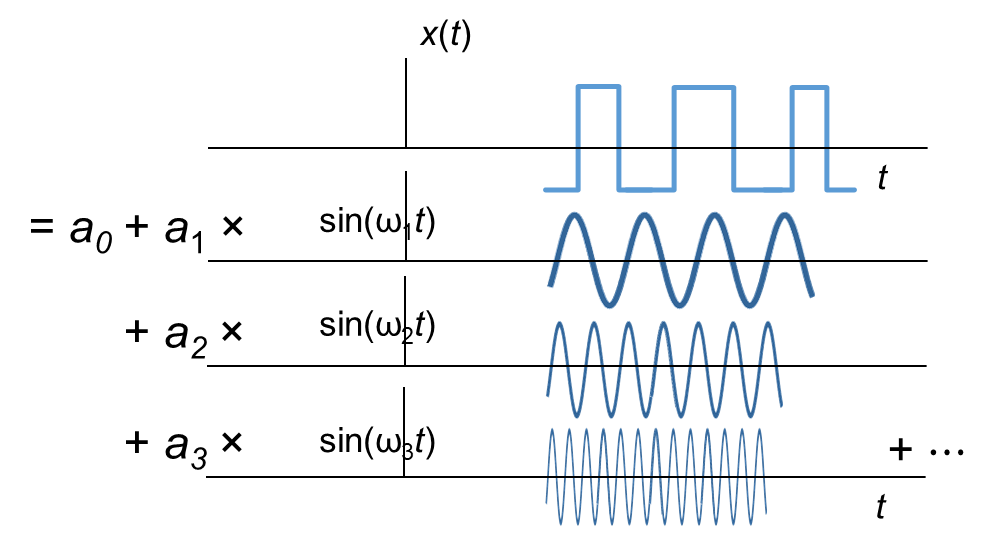
Fig 9: Fourier Series Credit: [Kyle Jamieson] (https://www.cs.princeton.edu/courses/archive/spring18/cos463/)
The frequency domain view is simply the weight vs the frequencies , showing the amount of power concentrated on each frequency.
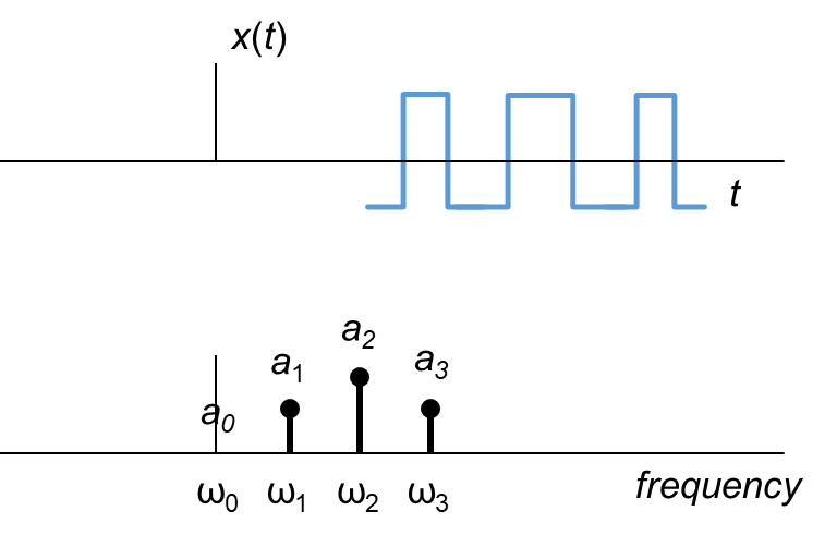
Fig 10: Frequency View Credit: [Kyle Jamieson] (https://www.cs.princeton.edu/courses/archive/spring18/cos463/)
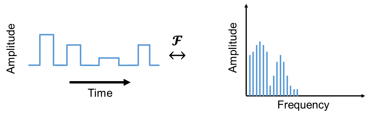
Fourier Transform
The Fourier Series deals with periodic signals. Not all signals are periodic, Fourier Transform deals with non-periodic signals.
Notation
Fourier Transform Pairs
Sampling
Nyquist Theorem
Definition
The sampling frequency should be at least twice the highest frequency contained in the signal.
where is sampling frequency and is the highest frequency contained in signal.
Fourier Transform of the Impulse Train
Let us have a quick look at what is happening here, use angular frequency . The impulse train has Fourier transform (a standard result):
where
Equivalently, in ordinary frequency :
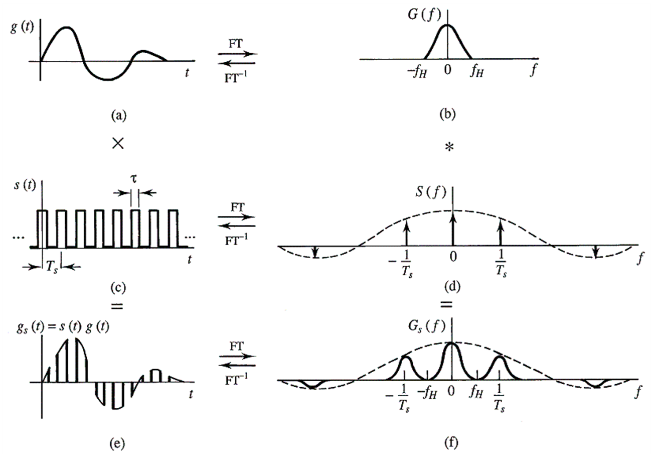
Fourier Transform of the Sampled Signal — Convolution in Frequency
Multiplication in time convolution in frequency.
Let
Then
Substituting :
So:
That is, the spectrum of the sampled signal is the original spectrum repeated (shifted) by integer multiples of , scaled by .
In Ordinary Frequency (Hz)
If we use with :
(Here there is no scaling in the -domain because of the Fourier transform normalization. Both forms are equivalent if you use consistent conventions.)
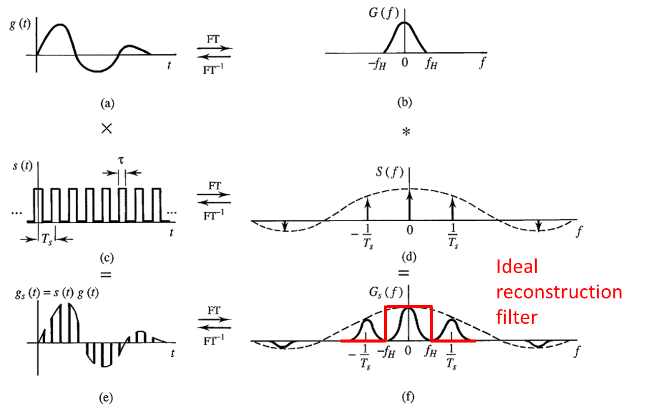
Interpretation — Aliasing and Nyquist
If is bandlimited to and (equivalently ), the shifted spectra do not overlap. The original spectrum can be recovered by lowpass filtering and scaling. If (or ) is too small, the shifted spectra overlap resulting in aliasing.
Short Summary
Sampling in time:
Spectrum of impulse train:
Spectrum of sampled signal:
Natural Sampling
- Original continuous signal recovered from its samples by separating its original baseband spectrum from its higher frequency spectral replicas
- Filter used is called a reconstruction filter
Aliasing
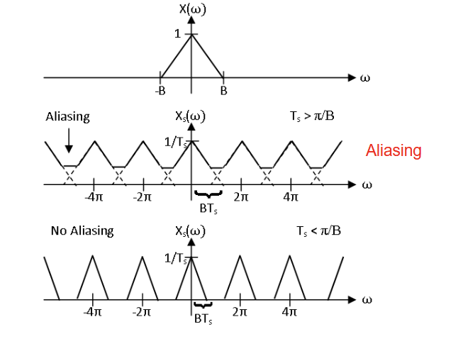
- Antialiasing filter located immediately prior to sampling circuit
- Antialiasing filter limits frequencies in pre-sampled signal to half the sampling rate (folding frequency) thus preventing aliasing
- To avoid amplitude (and phase) distortion amplitude response should be flat across the bandwidth of signal (and phase response must be linear)
- To minimise aliasing filter must have sufficiently rapid roll-off and sufficient attenuation above the cut-off (i.e. folding) frequency