Lecture 2 - Part 2

Sensor Data
Types of Sensors
Regression in Time-Series Analysis
Types of Regression

Sensor Data

The form and the nature of data provided by sensors differ based on their type. A few data formats that are commonly encountered in Edge AI applications are as follows:

Time Series

Time series data represents how a variables of interest changes over time. A single sensor can produce multiple time-series data streams. For instance consider an environmental sensor (e.g. BME680) it may provides measurement for temperature, humidity, pressure, and gas levels.
Typically, time series data is collected by polling the sensors with a certain frequency. Ironically, this frequency is also called sampling frequency and the rate of polling, i.e. number of samples collected per second is known as sampling rate.
Note that this sampling rate is not same as the sampling rate we discussed in A/D conversion. Key differences have been articulated in table below.
Some time series are aperiodic, meaning samples are not taken at fixed intervals. This occurs with sensors that respond to specific events, such as a proximity sensor that triggers when an object enters a defined range. In such cases, it is common to record the exact timestamp along with the sensor reading.
Time series can also represent aggregated information, such as the number of occurrences of an event within a given time interval.

Key Differences: Time Series Sampling vs Physical Signal Sampling

Aspect	Physical Signal Sampling (ADC)	Time Series Sampling (Digital)
Domain	Continuous-time, continuous-amplitude	Discrete-time, already digital
Purpose	Convert real-world signal to digital	Reduce, resample, or analyze data
Sampling Constraint	Must satisfy Nyquist criterion	No strict Nyquist limit
Data Source	Sensor measuring physical quantities	Pre-recorded or generated digital data
Sampling Rate	Determined by highest frequency in signal	Determined by analysis or polling requirements
Examples	Microphone recording sound at 44.1 kHz	Stock prices sampled daily or hourly
Event Handling	Typically continuous measurement	Can be periodic or aperiodic (event-driven)
Tools	Sensor + ADC hardware	Software or algorithms

Signal Modality

Audio Signals

An audio signal captures oscillation of sound waves traveling in a certain medium (air, water, vacuum, etc.). Audio signals are also example of time series data. Audio signals capture changes in air pressure over time. Generally, audio signals are sampled with very high frequency. The upper limits to human hearing are around 20 kHz. Consequently, from Nyquist Theorem, audio signals must be captured at twice the rate, i.e., 40 kHz. With each sample, using ADC $N=8$ , we have 320Kbps. The Ultrasonic signals which can be used to measure density of liquid or other liquid properties go beyond this audible range. Audio signals can also yield multiple time series, specially for stereo audio. However, for sake of simplicity, let us restrict ourselves to mono-audio. Then the discrete-time audio signal can be represented as a column vector:

\mathbf{x} = \begin{bmatrix} x[0] \\ x[1] \\ x[2] \\ \vdots \\ x[N-1] \end{bmatrix}

where:

$\mathbf{x}$ is the vector of audio samples,
$x[n]$ is the amplitude of the $n$ -th sample,
$N$ is the total number of samples.

Image Signals

An image sensor is a device that captures light from a scene and converts it into electrical signals. Common types include CCD (Charge-Coupled Device) and CMOS (Complementary Metal-Oxide-Semiconductor). The sensor consists of a 2D array of photosensitive elements called pixels, where each pixel measures the intensity of light hitting it and converts it into a digital value. The digital output of an image sensor can be represented as a matrix where each element corresponds to a pixel value. For a grayscale image, the matrix is written as:

I = \begin{bmatrix} I[0,0] & I[0,1] & \cdots & I[0,N-1] \\ I[1,0] & I[1,1] & \cdots & I[1,N-1] \\ \vdots & \vdots & \ddots & \vdots \\ I[M-1,0] & I[M-1,1] & \cdots & I[M-1,N-1] \end{bmatrix}

where $I[m,n]$ is the intensity of the pixel at row $m$ and column $n$ , $M$ is the number of rows, and $N$ is the number of columns. For color images, each pixel contains multiple components (e.g., RGB), so the image can be represented as a 3D array $I[m,n,c]$ where $c \in \{R, G, B\}$ .Similarly, Radio detection and ranging (radar) and LiDAR systems generate spatial imaging data, which can also be represented as matrices or 3D arrays, where each element corresponds to a measured intensity, distance, or reflectivity value at a specific spatial location.

Select an image:

The image will be available in Python as window.imgData.

Image Channels

Loading editor...

No output yet. Click "Run Python" to execute.

video

The Video data is essentially a collection of images sampled at what is known as frame rate. Videos can be encoded through efficient encoding scheme to reduce the storage size. Such encoding schemes also utilise temporal variations across the frames.

Types of Sensors

Category	What it does	Example
Acoustic & Vibration	• Measure vibrations traveling through a medium air (microphones) water (hydrophones) ground (geophones and seismometers) • Provides a time series describing the variation of pressure • Acoustic signals contain info across frequencies • High-frequency signals require high sample rates	Shure SM58 Microphone Geosense GS-11VT Seismometer
Visual and Scene	• Capture light using sensor arrays • Color channels: grayscale or RGB • Spectral response: visible and infrared • Pixel size: larger = more sensitive • Sensor resolution: more elements = finer detail • Frame rate: captures images per second	Sony IMX586 Image Sensor FLIR Lepton Thermal Camera
Motion and Position	• Tilt sensor: detects orientation • Accelerometer: measures acceleration • Gyroscope: measures rotation • Time of Flight: measures distance via EM emission • IMU: combines sensors to find position • GPS: uses satellites to locate device	Tilt Ball Switch ADXL345 MPU-6050 VL53L0X BNO055 u-blox NEO-6M
Force and Tactile	• Button & Switch: binary signal • Capacitive Touch: detects touch • Strain & Flex: measures deformation • Load Cells: measure applied load • Pressure Sensors: gas/liquid pressure • Flow Sensors: rate of flow	CherryMX MPR121 (NXP) Flex Sensor TAL220B BMP280 Honeywell AWM1700
Environmental & Others	• Temperature • Particulate Matter • Gas concentrations • Photo sensor: detects light • Bio signals: heart, brain, etc. • Chemical: measures specific chemicals	DS18B20 PMS5003 MQ-135 TSL2561 AD8232 Atlas Scientific pH Sensor

Regression in Time-Series Analysis

Having sampled the time-series data, we want to develop some basic understanding of physical phenomenon. Regression is a statistical method used to model the relationship between a dependent variable and one or more independent variables. In time-series analysis, regression can help us understand trends, make predictions, and quantify the influence of time or other factors on a variable.

Example:
We have daily temperature measurements over a month. We want to model the trend of temperature over time and potentially predict future values.

Time-Series Data

Suppose we have:

Day	Temperature (°C)
1	15
2	16
3	16.5
...	...
30	21

Independent variable $x$ : Day number (1 to 30)
Dependent variable $y$ : Temperature

We want a simple regression:

y = \beta_0 + \beta_1 x + \epsilon

Where:

$\beta_0$ = intercept (temperature at day 0)
$\beta_1$ = slope (rate of change of temperature per day)
$\epsilon$ = error term

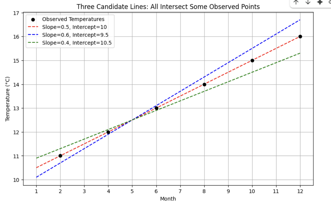
Least Squares Regression

Goal: Find $\beta_0$ and $\beta_1$ that minimize the sum of squared errors:

S(\beta_0, \beta_1) = \sum_{i=1}^{n} \big(y_i - (\beta_0 + \beta_1 x_i)\big)^2

This is called Ordinary Least Squares (OLS).

The closed-form solution for simple linear regression:

\beta_1 = \frac{\sum (x_i - \bar{x})(y_i - \bar{y})}{\sum (x_i - \bar{x})^2}, \quad \beta_0 = \bar{y} - \beta_1 \bar{x}

Where $\bar{x}$ and $\bar{y}$ are the sample means.

Solution Approach

To find the minimum, take derivatives with respect to $\beta_0$ and $\beta_1$ and set them to zero:

\frac{\partial S}{\partial \beta_0} = -2 \sum_{i=1}^n \big(y_i - \beta_0 - \beta_1 x_i\big) = 0

\frac{\partial S}{\partial \beta_1} = -2 \sum_{i=1}^n x_i \big(y_i - \beta_0 - \beta_1 x_i\big) = 0

Normal Equations

Simplifying the derivatives gives the normal equations:

\begin{cases} n \beta_0 + (\sum x_i)\beta_1 = \sum y_i \\ (\sum x_i)\beta_0 + (\sum x_i^2)\beta_1 = \sum x_i y_i \end{cases}

Solve for Slope $\beta_1$ by defining the means:

\bar{x} = \frac{1}{n} \sum x_i, \quad \bar{y} = \frac{1}{n} \sum y_i

Then the slope is:

\beta_1 = \frac{\sum_{i=1}^{n} (x_i - \bar{x})(y_i - \bar{y})}{\sum_{i=1}^{n} (x_i - \bar{x})^2}

Once $\beta_1$ is known, the intercept is:

\beta_0 = \bar{y} - \beta_1 \bar{x}

\boxed{ \beta_1 = \frac{\sum_{i=1}^{n} (x_i - \bar{x})(y_i - \bar{y})}{\sum_{i=1}^{n} (x_i - \bar{x})^2}, \quad \beta_0 = \bar{y} - \beta_1 \bar{x} }

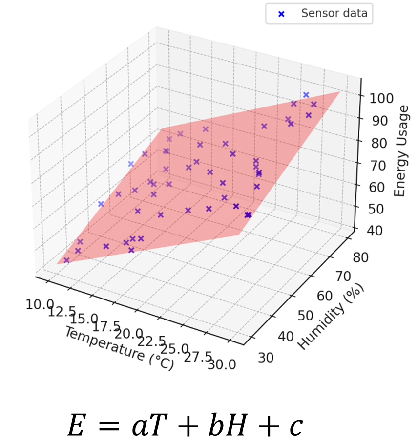
Types of Regression

Regression is a statistical technique used to model the relationship between a dependent variable (y) and one or more independent variables (x).

1. Linear Regression

Models the relationship as a straight line:

y = \beta_0 + \beta_1 x + \epsilon

Goal: Find coefficients $\beta_0, \beta_1$ that minimize the error.
Can be simple (one predictor) or multiple (many predictors).

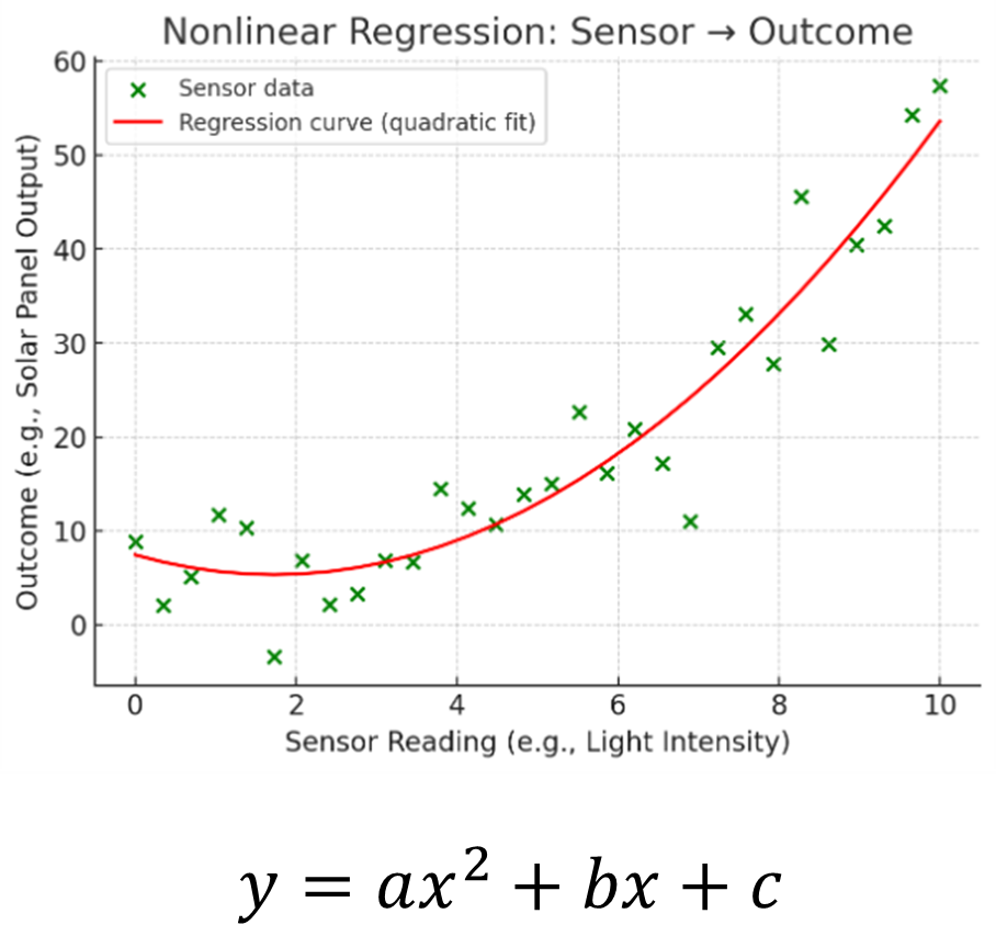
y = \beta_0 + \beta_1 x_1 + \beta_2 x_2 + \dots + \beta_p x_p + \epsilon

2. Polynomial Regression

Models the relationship using polynomials of degree $n$ :

y = \beta_0 + \beta_1 x + \beta_2 x^2 + \dots + \beta_n x^n + \epsilon

Captures non-linear trends.
Still solved with least squares.
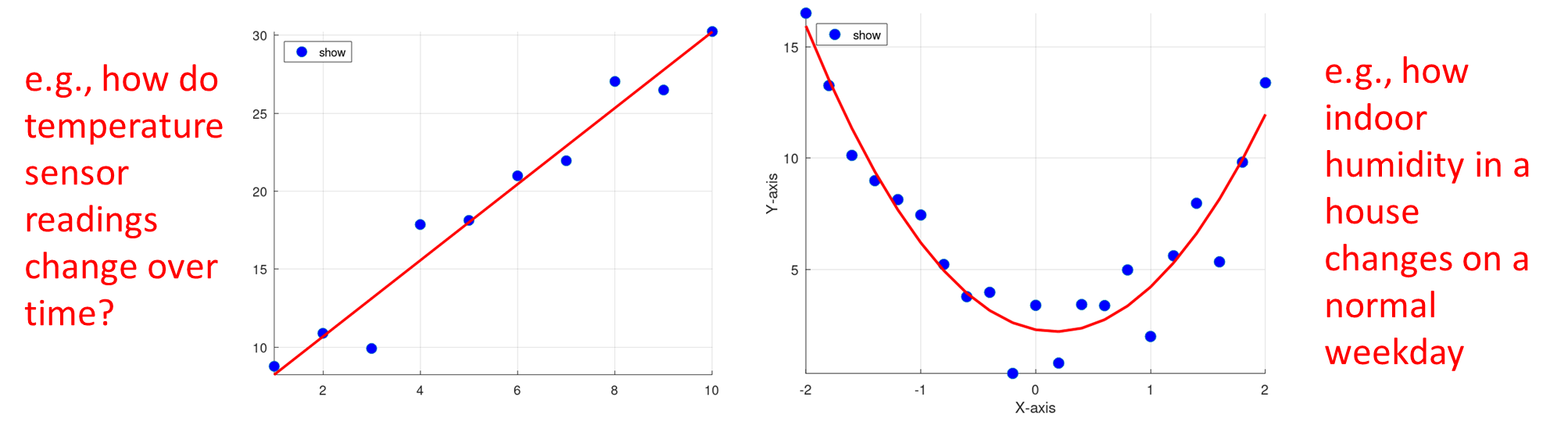
Imagine a solar panel on your roof. Early in the morning, with just a little sunlight, it barely produces any power. As the sun rises, output grows faster and faster, but after a point it starts to level off. The pattern isn’t a straight line, it curves

3. Logistic Regression

Used when the dependent variable is categorical (binary):

P(y=1|x) = \frac{1}{1 + e^{-(\beta_0 + \beta_1 x)}}

Models probabilities, not continuous outcomes.