Lecture 4 - Part 1

Contents

• Introduction to Detection
• Neyman-Pearson Criterion
  • Binary Hypothesis test
  • General Problem Setup for Detection of DC Buried in Noise
  • Likelihood Functions
  • Likelihood Ratio Test (LRT)
  • Neyman-Pearson Criterion
  • Receiver Operating Curve (ROC)
  • Generalization: Bayes Risk
    • Bayes Risk Formulation
    • Bayes Decision Rule
    • Special Cases
• References

Introduction to Detection

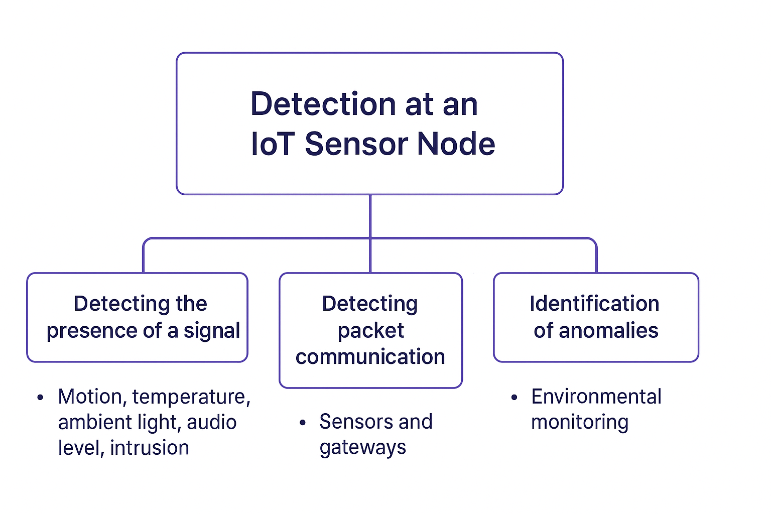
One of the key functionality at the IoT sensor node is to detect an event. The sensing tasks range from:

1. Detecting the motion, change in temperature, ambient light, intrusion or change in audio level. All these tasks are detecting the absence or presence of certain signal.
2. Detecting the packets sent to communicate these readings between a sensor and the gateway. In other words, we often need to detect the packets and then decode it to understand the values.
3. Identification of anomalies, e.g. in the environmental monitoring case (increase in CO, particulate matter levels etc.).

Detection of certain attributes also is key in triggering more complex processing operation. For instance, consider an audio IoT sensors deployed at scale in wild. These are deployed to detect presence of certain species of birds or animals [1]. Rather than capturing the sound and processing it continuously, often in the IoT systems (typically having multiple cores of MCUs), its customary to detect the sound first and then trigger the complex classification pipeline. This saves the unnecessary usage of battery on the sensors, increasing the operational life-time for the deployment.

A detection problem can be casted as a simple hypothesis testing problem. Under each hypothesis, the desired attribute follows a completely known distribution. The classical approach for the detection theory are based on Neyman-Pearson theorem and a Bayesian approach is based on Bayesian Risk Minimisation. When the distribution of the signal is not exactly known then energy detection can be employed. We will only explore these aspects alongside some representative use-cases where these will be employed in IoT deployments.

Neyman-Pearson Criterion

To appreciate Neyman-Pearson criterion, let us start with a very simple example of binary hypothesis testing. In other words, let us assume that we observe a single realisation (sample/instance) of a random variable whose PDF is either $\mathcal{N}(0,1)$ or $\mathcal{N}(1,1)$. Essentially, the hypothesis testing problem is to determine from single sample say $x[0] \sim \mathcal{N}(\mu,1)$ whether $\mu=1$ or $\mu=0$, i.e. which distribution it belongs to. Mathematically,

$$\begin{align} \mathcal{H}_0 &: \mu=0 \text{ or } x[0]=w[0] ,\\ \mathcal{H}_1 &: \mu=1 \text{ or } x[0]=s[0]+w[0],\\ & w[0] \sim \mathcal{N}(0,1) \text{ and } s[0] = 1, \end{align}$$

where $\mathcal{H}_0$ is referred to as the null hypothesis and $\mathcal{H}_1$ as the alternate hypothesis. The PDF under both hypothesis is shown below, with the difference in $\mu$ accounting for the shift to the right under $\mathcal{H}_1$. As you can see from the single sample it is difficult to detect which one of the distributions it belongs to specially given the overlap between them. The decision can be made on basis of fixed threshold. The threshold line is indicated by dashed black line. Drag the slider at the bottom of the figure to fix the threshold to $x[0]=0.5$.

This presents one possible approach, i.e., if $x[0]>\frac{1}{2}$ then its more likely for $x[0]\in \mathcal{H}_1$, therefore hypothesis $\mathcal{H}_1$ is true. Alternatively, we can say if $x[0]>\frac{1}{2}$ then $p(x[0]|\mathcal{H}_1)>p(x[0]|\mathcal{H}_0)$. So the detection model is simply comparing the observed $x[0]$ with a threshold, i.e., say $\gamma=\frac{1}{2}$. With this approach we can make two type of errors:

1. If we decide $\mathcal{H}_1$ instead of $\mathcal{H}_0$, we make Type I error. The probability of making Type I error, i.e., say $P(\mathcal{H}_1\vert \mathcal{H}_0)$ is known as Probability of False Alarm and is denoted by $P_{FA}$.
2. If we decide $\mathcal{H}_0$ instead of $\mathcal{H}_1$, we make Type II error. The probability of making Type II error, i.e., say $P(\mathcal{H}_0\vert \mathcal{H}_1)$ is known as Probability of Missed Detection and is denoted by $P_{MD}$. The probability of missed detection is $P_{MD}=1-P_{D} =1-P(\mathcal{H}_1\vert \mathcal{H}_1)$.

As you will notice from the figure above, it is not possible to reduce both error probabilities simultaneously. Reducing one increases the other, i.e., there is inherent trade-off between $P_{FA}$ and $P_{MD}$. Consequently, a sensible approach to designing optimal detector is to hold one of these probabilities constant while minimising the other. For instance, fix $P_{FA}=\epsilon$, with $\epsilon$ being small constant while minimising the $P_{MD}$.

What the formula says is given $L(\boldsymbol{x})$ is the likelihood ratio:

• If it’s larger than the threshold $\gamma$, we decide $\mathcal{H}_1$ (signal present).
• Otherwise, we decide $\mathcal{H}_0$ (signal absent).

The threshold is not arbitrary—it is chosen so that the probability of false alarm equals a predefined level $\epsilon$. Lastly, the

$$P_{FA} \;=\; \int_{\{\boldsymbol{x} : L(\boldsymbol{x}) > \gamma\}} p(\boldsymbol{x} \mid H_{0}) \, d\boldsymbol{x} \;=\; \epsilon$$

This integral means: we add up the probability mass of all outcomes $x$ that would make us mistakenly decide $\mathcal{H}_{1}$, when $\mathcal{H}_{0}$ is in fact true. That probability must equal $\epsilon$, which is a design parameter (for example, $(\epsilon = 10^{-3})$).

Binary Hypothesis test

For the hypothesis test of the problem we introduced above, we can easily find the NP test. Assume that we require $P_{FA} = 10^{-3}$. Then, from $L(\boldsymbol{x})$ we decide $\mathcal{H}_{1}$ if

$$\frac{p(\boldsymbol{x} \vert \mathcal{H}_{1})}{p(\boldsymbol{x} \vert \mathcal{H}_{0})} = \frac{\tfrac{1}{\sqrt{2\pi}} \exp\!\left[-\tfrac{1}{2}(x[0]-1)^{2}\right]} {\tfrac{1}{\sqrt{2\pi}} \exp\!\left[-\tfrac{1}{2}x^{2}[0]\right]} > \gamma$$

or

$$\exp\!\left[-\tfrac{1}{2}\left(x^{2}[0] - 2x[0] + 1 - x^{2}[0]\right)\right] > \gamma$$

or finally

$$\exp\!\left(x[0] - \tfrac{1}{2}\right) > \gamma.$$

At this point we could determine $\gamma$ from the false alarm constraint

$$P_{FA} = P\!\left\{ \exp\!\left(x[0]-\tfrac{1}{2}\right) > \gamma \;\middle|\; \mathcal{H}_{0} \right\} = 10^{-3}.$$

A simpler approach is to take logarithms (since log is monotonic). So we decide $\mathcal{H}_{1}$ if

$$x[0] > \ln \gamma + \tfrac{1}{2}.$$

Letting $\gamma' = \ln \gamma + \tfrac{1}{2}$, we decide $\mathcal{H}_{1}$ if $x[0] > \gamma'$. To explicitly find $\gamma'$ we use the $P_{FA}$ constraint:

$$P_{FA} = P\{ x[0] > \gamma' \mid \mathcal{H}_{0} \} = \int_{\gamma'}^{\infty} \frac{1}{\sqrt{2\pi}} \exp\!\left[-\tfrac{1}{2}x^{2}\right] \, dx = 10^{-3}.$$

Thus $\gamma' = 3$. The NP test is to decide $\mathcal{H}_{1}$ if $x[0] > 3$. The detection probability is then

$$P_{D} = P\{ x[0] > 3 \mid \mathcal{H}_{1} \} = \int_{3}^{\infty} \frac{1}{\sqrt{2\pi}} \exp\!\left[-\tfrac{1}{2}(x-1)^{2}\right] \, dx = 0.023.$$

If instead we require $P_{FA} = 0.5$, then the threshold is found from

$$0.5 = \int_{\gamma'}^{\infty} \frac{1}{\sqrt{2\pi}} \exp\!\left[-\tfrac{1}{2}x^{2}\right] \, dx$$

which gives $\gamma' = 0$. Then

$$P_{D} = \int_{0}^{\infty} \frac{1}{\sqrt{2\pi}} \exp\!\left[-\tfrac{1}{2}(x-1)^{2}\right] \, dx = \int_{0}^{\infty} \frac{1}{\sqrt{2\pi}} \exp\!\left[-\tfrac{1}{2}(x^{2} - 2x + 1)\right] \, dx. =1-Q(1)=0.84.$$

This essentially shows that you can trade the higher $P_D$ for tolerating higher $P_{FA}$.

General Problem Setup for Detection of DC Buried in Noise

Consider the binary hypothesis testing problem:

$$\begin{align} \mathcal{H}_0: &\quad x[n] = w[n] \quad \text{(noise only)} \\ \mathcal{H}_1: &\quad x[n] = A + w[n] \quad \text{(signal + noise)} \end{align}$$

where:

• $x[n]$ is the observed signal at time $n$
• $A$ is a known constant amplitude
• $w[n] \sim \mathcal{N}(0, \sigma^2)$ is additive white Gaussian noise

For $N$ observations $\mathbf{x} = [x[0], x[1], \ldots, x[N-1]]^T$, the hypotheses become:

$$\begin{align} \mathcal{H}_0: &\quad \mathbf{x} = \mathbf{w} \\ \mathcal{H}_1: &\quad \mathbf{x} = A\mathbf{1} + \mathbf{w} \end{align}$$

where $\mathbf{1} = [1, 1, \ldots, 1]^T$ and $\mathbf{w} \sim \mathcal{N}(\mathbf{0}, \sigma^2\mathbf{I})$.

Likelihood Functions

Under each hypothesis, the likelihood functions are:

$$\begin{align} p(\mathbf{x}|\mathcal{H}_0) &= \frac{1}{(2\pi\sigma^2)^{N/2}} \exp\left(-\frac{1}{2\sigma^2}\sum_{n=0}^{N-1} x[n]^2\right) \\ p(\mathbf{x}|\mathcal{H}_1) &= \frac{1}{(2\pi\sigma^2)^{N/2}} \exp\left(-\frac{1}{2\sigma^2}\sum_{n=0}^{N-1} (x[n] - A)^2\right) \end{align}$$

Likelihood Ratio Test (LRT)

The likelihood ratio is:

$$L(\mathbf{x}) = \frac{p(\mathbf{x}|\mathcal{H}_1)}{p(\mathbf{x}|\mathcal{H}_0)} = \exp\left(\frac{A}{\sigma^2}\sum_{n=0}^{N-1} x[n] - \frac{NA^2}{2\sigma^2}\right)$$

Taking the natural logarithm:

$$\ln L(\mathbf{x}) = \frac{A}{\sigma^2}\sum_{n=0}^{N-1} x[n] - \frac{NA^2}{2\sigma^2}$$

The LRT decision rule is:

$$\ln L(\mathbf{x}) \begin{cases} > \ln \gamma & \text{decide } \mathcal{H}_1 \\ < \ln \gamma & \text{decide } \mathcal{H}_0 \end{cases}$$

This simplifies to the test statistic:

$$T(\mathbf{x}) = \sum_{n=0}^{N-1} x[n] \begin{cases} > \gamma' & \text{decide } \mathcal{H}_1 \\ < \gamma' & \text{decide } \mathcal{H}_0 \end{cases}$$

where $\gamma' = \frac{\sigma^2 \ln \gamma}{A} + \frac{NA}{2}$.

Neyman-Pearson Criterion

The Neyman-Pearson lemma states that for a given probability of false alarm $P_{FA} = \alpha$, the likelihood ratio test maximizes the probability of detection $P_D$ (or equivalently, minimizes the probability of missed detection).

For our problem:

• Under $H_0$: $T(\mathbf{x}) \sim \mathcal{N}(0, N\sigma^2)$
• Under $H_1$: $T(\mathbf{x}) \sim \mathcal{N}(NA, N\sigma^2)$

The probability of false alarm is:

$$P_{FA} = P(T > \gamma' | \mathcal{H}_0) = Q\left(\frac{\gamma'}{\sqrt{N}\sigma}\right)\\ \frac{\gamma'}{\sqrt{N}\sigma}=Q^{-1}(P_{FA})$$

The probability of detection is:

$$P_D = P(T > \gamma' | \mathcal{H}_1) = Q\left(\frac{\gamma' - NA}{\sqrt{N}\sigma}\right)\\ = Q\left(Q^{-1}(P_{FA})-{\frac{\sqrt{N}A}{\sigma}}\right)$$

where $Q(\cdot)$ is the Q-function (complement of the standard normal CDF). The value $\text{ENR}= N\frac{A^2}{\sigma^2}$ is often known as Energy-to-noise-ratio (can be expresed in dB scale as $10\log_{10}(\text{ENR})$). The figure below studies impact of varying ENR on $P_D$ for various $P_{FA}$'s.

Receiver Operating Curve (ROC)

A Receiver Operating Characteristic (ROC) curve is a graphical tool used to evaluate the performance of a binary classifier system by illustrating the trade-off between $P_D$ and $P_{FA}$ across different decision thresholds. Each point on the curve corresponds to a particular threshold, showing how increasing sensitivity (detecting more true positives) often comes at the cost of increased false alarms. The ROC curve provides a comprehensive view of a system’s discriminative ability, with curves closer to the top-left corner indicating better performance. The diagonal line $P_D=P_{FA}$ represents random guessing.

Generalization: Bayes Risk

The Neyman-Pearson approach fixes $P_{FA}$ and maximizes $P_D$. A more general approach is to minimize the Bayes risk, which considers the costs of different decision outcomes and prior probabilities.

Bayes Risk Formulation

Let:

• $C_{ij}$ = cost of deciding $H_i$ when $H_j$ is true
• $P(H_0)$, $P(H_1)$ = prior probabilities

The average risk is:

$$R = C_{00}P(H_0)P(\text{decide }H_0|H_0) + C_{01}P(H_0)P(\text{decide }H_1|H_0) + C_{10}P(H_1)P(\text{decide }H_0|H_1) + C_{11}P(H_1)P(\text{decide }H_1|H_1)$$

Typically, we assume $C_{00} = C_{11} = 0$ (correct decisions have no cost), so:

$$R = C_{01}P(H_0)P_{FA} + C_{10}P(H_1)P_{MD}$$

where $P_{MD} = 1 - P_D$ is the probability of missed detection.

Bayes Decision Rule

The Bayes optimal decision rule minimizes the expected risk:

$$\frac{p(\mathbf{x}|H_1)}{p(\mathbf{x}|H_0)} \begin{cases} > \frac{C_{01}P(H_0)}{C_{10}P(H_1)} & \text{decide } H_1 \\ < \frac{C_{01}P(H_0)}{C_{10}P(H_1)} & \text{decide } H_0 \end{cases}$$

This shows that the optimal threshold depends on:

1. The cost ratio $C_{01}/C_{10}$
2. The prior probability ratio $P(H_0)/P(H_1)$

Special Cases

Equal costs and priors: $C_{01} = C_{10}$, $P(H_0) = P(H_1) = 0.5$ Threshold = 1 (decide based on which hypothesis is more likely)

Minimax criterion: Choose the threshold to minimize the maximum possible risk

Neyman-Pearson: Equivalent to Bayes with specific cost assignments

The Bayes framework provides a unified approach that encompasses the Neyman-Pearson criterion as a special case, while allowing for incorporation of prior knowledge and decision costs.

References

[1] Pringle, S., Dallimer, M., Goddard, M.A. et al. Opportunities and challenges for monitoring terrestrial biodiversity in the robotics age. Nat Ecol Evol 9, 1031–1042 (2025). https://doi.org/10.1038/s41559-025-02704-9

[2] Kay, Steven M. Fundamentals of statistical signal processing: Detection theory. Prentice-Hall, Inc., 1993.