
Lecture 4 - Part 2
Contents
- Introduction
- Practical Aspects
- Zooming Out
- Networked Detection Perspective
- References
Introduction
In this chapter, we will first explore an interactive practical demo to see applicability of what we have learn so-far. We will then zoom out a bit and understand practical workflow involved in implementing detection on the IoT devices. Lastly, we will cover some advanced aspects of IoT when we are no-longer concerned about point observations and indeed want to capture spatio-temporal phenomenon using network of sensors.
Practical Aspects
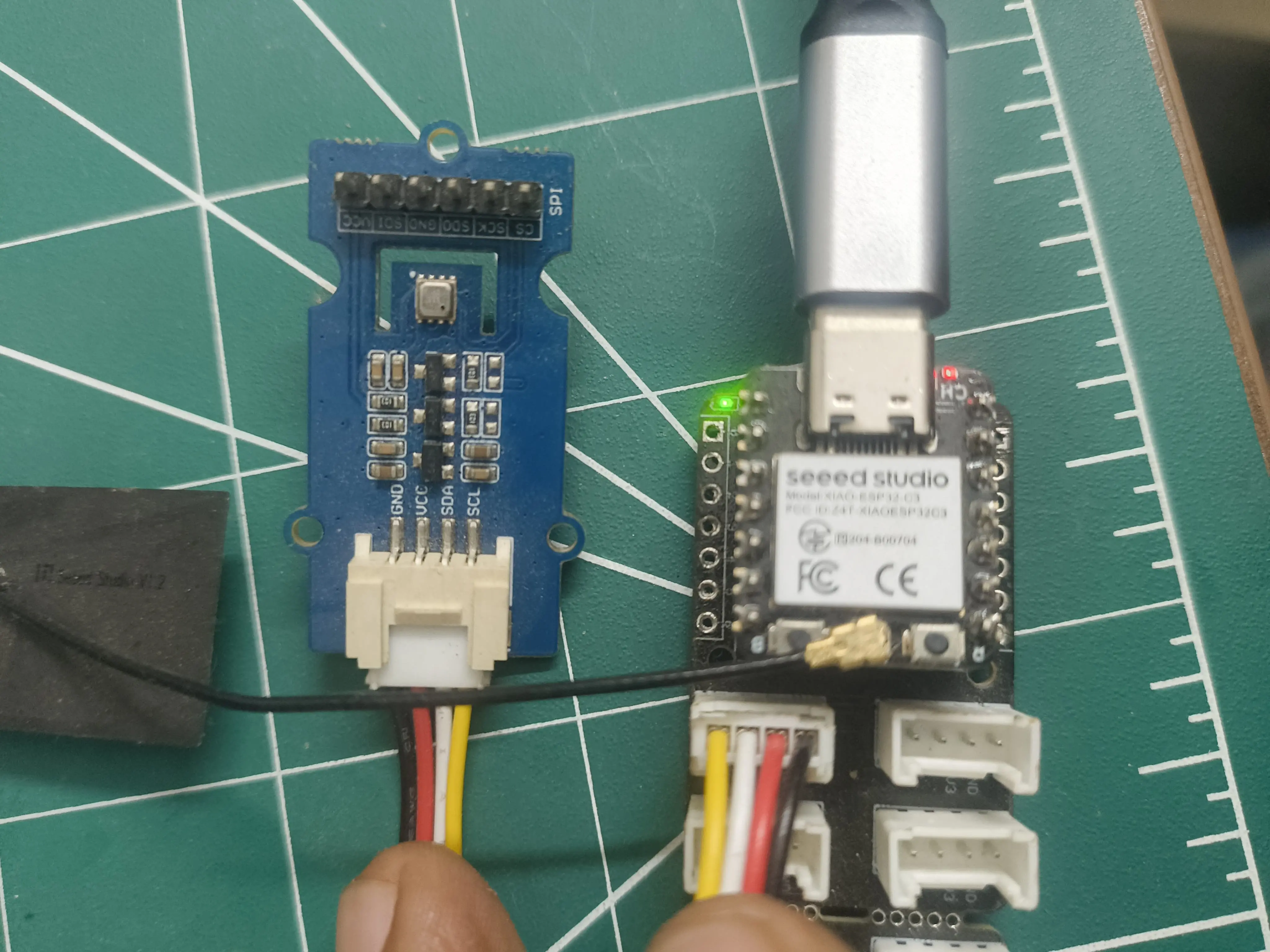
To test this demo, you need the board connected to the PC. You also need the right firmware on the board. The firmware tab has all the firmware detail. Once you have got the main.py and the drivers for BME680 on the board, you will be able to use I2C protocol to read sensor observations. A simple demo would involve detecting when sensor is hot vs. when it is at normal room temperature. To collect the data, first make connection and then press "Start". Once you have enough samples for "H₀" then from drop down switch to "H₁" and simultaneously either bring heat source close to sensor or spray a perfume etc. Once you are happy with number of samples under alternative hypothesis press stop and run the python script. You will be able to see the histogram.Now using the PDF you can fit a theoretical PDF and workout the NP criterion. The python editor is only enabled when you have data. You can see the readings for the data in the console tab.
Zooming Out
Having looked at the demo, now let us zoom out slightly. Let us understand the workflow for implementing the optimum detection, in a sense that its constant false alarm rate (CFAR). The flow chart below shows the steps involved. As you will observe, there are three stages. Data collection, determination of the optimal threshold, and lastly use of this threshold for inference.
Same workflow also applies when we have regression problem on the sensor observation rather than the detection.
Regression is one of the methods for time-series analysis and you will study this in quite some details within your ML courses. We will also cover some aspects of time-series processing in next few chapters.
Networked Detection Perspective
1. Introduction
In distributed detection, multiple sensors are deployed across a field to observe a physical phenomenon, such as temperature, moisture, or gas concentration. The goal is to combine these observations to make a reliable global decision.
Field Phenomenon Observation Diagram:
Sensors measure local signals which may be noisy, and send either raw measurements or local decisions to a central fusion center.
2. Problem Formulation
Binary hypothesis testing:
Each sensor observes and reports either:
- Raw observation → Data Fusion
- Local decision → Decision Fusion
The fusion center makes a global decision .
3. Data Fusion (Fusion of Raw Observations)
Data Fusion refers to the process where each sensor sends its raw measurement directly to a central fusion center. The fusion center then processes all the sensor observations collectively to make a global decision. This method is considered optimal because it retains all available information from the sensors, allowing the fusion center to compute the likelihoods of different hypotheses based on the full set of data.
Advantages of data fusion:
- Optimal performance: Uses all available information.
- Noise weighting: Sensors with lower noise can be given higher weights.
- Flexibility: Supports likelihood-based methods, Bayesian fusion, or weighted averaging.
Disadvantages:
- High bandwidth requirement: Raw sensor data must be transmitted.
- Centralized processing: Fusion center must handle all computations.
In essence, data fusion leverages the complete statistical information from all sensors to improve the reliability of the global decision, especially when sensor noise characteristics are known.
3.1 Ideal Scenario: Data Fusion
In the ideal scenario, all sensors provide perfect, noise-free measurements. Each sensor sends its raw observation to the fusion center, which can then perform exact statistical processing without any uncertainty due to sensor noise.
- Perfect measurements: Sensor readings exactly reflect the underlying signal.
- Optimal likelihood ratio test (LRT):
- Outcome: Fusion center can make error-free or near-perfect global decisions.
- Bandwidth requirement: All raw data must be transmitted.
3.2 Noisy Scenario: Data Fusion
In real-world scenarios, sensor measurements are often corrupted by noise. Each sensor observes:
- Effect of noise: Raw sensor readings are no longer perfect, reducing the discriminative power of the global likelihood ratio.
- Weighted fusion: Fusion center can assign weights based on noise variance:
- Outcome: Data fusion remains optimal in a statistical sense, but accuracy depends on noise levels and correct weighting.
- Bandwidth requirement: Still requires all raw data to be transmitted.
4. Decision Fusion (Fusion of Local Decisions)
Decision refers to the process where each sensor makes a local decision (e.g., a 1-bit binary decision) based on its own observation and sends only this decision to the fusion center. The fusion center then combines these local decisions using rules such as majority voting, OR, or AND to reach a global decision.
Advantages:
- Low bandwidth: Only 1-bit decisions per sensor need to be transmitted.
- Simplicity: Reduces computational load at the fusion center.
Disadvantages:
- Suboptimal performance: Some information is lost because the raw measurements are not transmitted.
- Sensitivity to local errors: If local sensors are noisy, their decisions can degrade global performance.
In practice, decision fusion is often preferred in resource-constrained networks where bandwidth and energy consumption are critical, but it is generally less accurate than data fusion because it cannot exploit the full statistical information from the sensors.
4.1 Ideal Observations
In the ideal scenario, each sensor makes a perfect local decision:
- Local detection probability:
- Local false alarm probability:
OR Rule
- Global misdetection probability:
- Description: Fusion center declares event present if any sensor detects it; minimizes misdetection. Also, equivalent to the complement of the union of detection events:
AND Rule
- Global misdetection probability:
- Description: Fusion center declares event present only if all sensors detect it; conservative approach.
Majority Voting Rule
- Global misdetection probability:
- Description: Event is declared present if more than half the sensors detect it; balanced rule between OR and AND.
4.2 Noisy Observations
Noise increases local errors ( decreases, increases)
5. Comparison Table
| Feature | Data Fusion | Decision Fusion |
|---|---|---|
| Data transmitted | Raw observations | Local 1-bit decisions |
| Performance | Optimal ideal | Suboptimal |
| Noise handling | Weighted fusion improves robustness | Only mitigated via fusion rule or soft decisions |
| Bandwidth | High | Low |
6. Summary
- Distributed detection uses multiple sensors to improve reliability.
- Data fusion is optimal but bandwidth-intensive.
- Decision fusion is simpler and low-bandwidth but suboptimal.
- Noise reduces accuracy; data fusion can partially compensate via weighting, decision fusion suffers more from local errors.
References
[1] Ross, "Signal Processing for Communications", EPFL Press, 2008.