
Lecture 6- Part 1
Contents
- Machine Learning
- Traditional Approach vs Machine Learning Workflow
- Classification of ML Systems
- Main Challenges of ML
- Bias vs Variance Tradeoff
- Training and Validation of Models
- References
Machine Learning
What is ML and Why Learn ML?
Machine Learning (ML) is science and art of programming so that computers can learn patterns from data and make predictions or decisions without being explicitly programmed for every task.
Definition
A computer program is said to learn from experience E with respect to some task T and some performance measure P, if its performance on T, as measured by P, improves with experience E.
Tom Mitchell, 1997
Mathematically, this can be described as
Where:
- = input features (sensor readings, images, text, etc.)
- = target output (class labels, future value, anomaly detection)
- = learned model that predicts from
Core Idea:
Instead of coding rules explicitly, the model learns patterns from examples. The collection of examples used to train the system is called the training set. Each individual example (or instance) drawn from the training set is called a sample.
To evaluate how well the model has learned, some portion of data is held out as a testing set (or validation set). If the model has successfully captured the underlying function then its performance on the testing set should be similar to its performance on the training set. Large differences usually indicate overfitting (the model memorized training data) or underfitting (the model is too simple).
Example:
- Predicting temperature from sensor data
- Detecting if a machine is failing based on vibration readings
Traditional Approach vs Machine Learning Workflow
Traditional Programming
In Traditional Programming, the system’s behavior is explicitly defined by human-written rules or signal processing (SP) algorithms. Input data flows through these rules to produce an output / decision (see left diagram above). In contrast, Machine Learning for Edge AI allows the system to learn patterns from data rather than relying solely on hand-crafted rules. The workflow starts with collecting IoT / sensor data, followed by preprocessing and feature engineering, then moves to model training (on cloud or edge), followed by evaluation on a test set, optimization for edge devices, deployment, and finally on-device inference or prediction (see right diagram).
Despite the rise of ML, hybrid approaches that combine signal processing with ML remain highly relevant. For example, in IoT applications, SP techniques such as filtering, FFT, or feature extraction can reduce noise, highlight important patterns, and compress raw data before it is fed into a machine learning model. This improves model performance, increases robustness, and reduces computational and memory requirements, which is critical for resource-constrained edge devices. Such hybrid systems leverage the strengths of both paradigms: the interpretability and efficiency of SP and the adaptability of ML.
Machine Learning / Edge AI
Classification of ML Systems
Machine Learning (ML) systems can be classified in multiple ways, depending on the learning paradigm, output type, learning strategy, training mode or deployment context. Understanding these classifications helps in selecting the right ML approach for IoT and Edge AI applications.
Learning Paradigm
ML models can be classified through the lens of the degree of supervision required during training. Depending on how much guidance is provided, i.e. from full supervision to none. ML systems are typically categorized into four groups: supervised learning, unsupervised learning, semi-supervised learning, and reinforcement learning.
Supervised Learning
In supervised learning, the training data we expose to our ML system also includes desired outcomes, often called labels. In other words the system learn a mapping by considering inputs and associated labels .
Typical examples include regression and classification. Regression is geared towards predicting a target numeric value given a set of features, often also called predictors. Classification involves learning the decision boundaries for each class from the labelled data-set. These boundaries can then be used to assign class to previously un-seen data points. Supervised learning is widely used in Edge AI for on-device predictions.
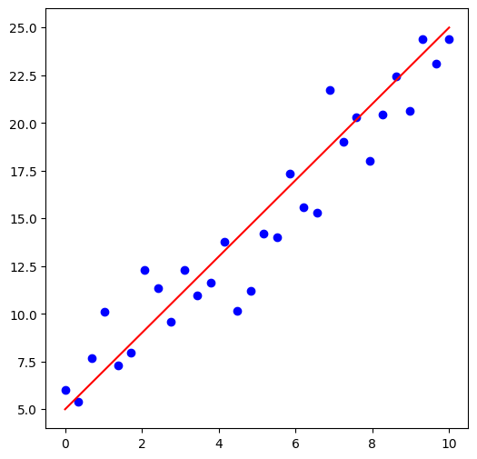
Example of Regression
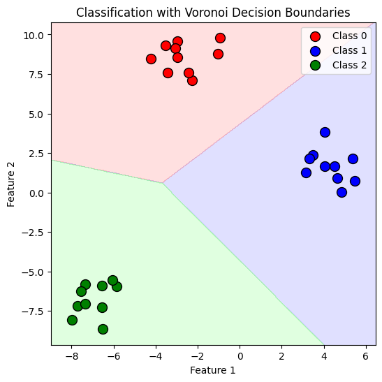
Example of Classification
There are several well-known supervised learning techniques, e.g., k-Nearest Neighbors, Linear Regression, Logistic Regression, Support Vector Machines (SVMs), Decision Trees and Random Forests, and lastly the Neural networks (NNs). Similarly, there are several un-supervised learning techniques mainly focused around clustering and dimensionality reduction. Given that ML itself requires multiple courses, we will treat the topic broadly. However, for your projects feel free to deep dive into these topics.
Unsupervised Learning
Contrary to supervised learning, unsupervised learning uses unlabelled training data. The ML system must therefore infer the underlying structure or distribution of the data, e.g., by performing clustering on the feature set, or by identifying which features (or combinations of features) help distinguish between dissimilar data points.
Common unsupervised learning methods include k-means clustering, hierarchical clustering, and dimensionality reduction techniques such as Principal Component Analysis (PCA). These approaches are widely used in IoT and Edge AI for pattern discovery, anomaly detection, and feature compression.
Example: In IoT systems, large numbers of sensors generate continuous streams of data, such as temperature, humidity, or vibration readings. Often, these data are unlabelled, especially during initial deployment or in large sensor networks. Unsupervised learning, such as K-Means clustering, can automatically detect patterns, operational modes, or anomalies without requiring prior labels.
For example, an edge device monitoring environmental conditions in a smart building can use clustering to discover:
-
Regions or rooms with similar temperature-humidity profiles,
-
Operating patterns (e.g., occupied vs. unoccupied zones), or
-
Unexpected sensor behaviour indicating faulty readings or abnormal use.
The example below simulates IoT temperature-humidity data from multiple rooms and applies K-Means clustering to uncover natural groupings in the data without explicit labels.
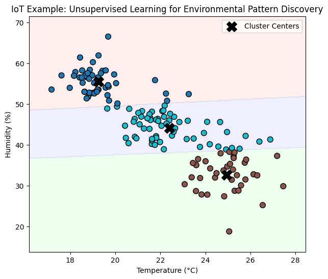
Example of Unsupervised Learning using K-means.
Visualisation techniques which plot data samples against reduced feature set can also provide great insight into classifying the data.
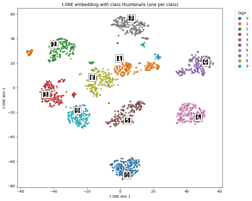
Visualisation using t-SNE Embedding on Digits 0-9.
A related task in IoT data analytics is dimensionality reduction, where the goal is to simplify high-dimensional sensor data while preserving the most important information. This is especially useful for resource-constrained edge devices, which must process or transmit data efficiently.
One common approach is to merge correlated sensor readings into a single, more informative feature. For example, temperature and humidity readings from an indoor sensor node are often highly correlated — a dimensionality reduction algorithm such as Principal Component Analysis (PCA) can combine them into a single latent feature representing the overall thermal comfort level.
This process of creating new, compact features from existing ones is known as feature extraction, and it helps reduce bandwidth, computation, and energy usage in IoT systems while retaining essential patterns for further analysis or prediction.
Semi-supervised Learning
Semi-supervised learning lies between supervised and unsupervised learning.
It leverages a small amount of labeled data and a large pool of unlabeled data to improve learning accuracy.
This approach is particularly valuable in IoT and Edge AI systems, where collecting and labeling data (e.g., sensor fault states, activity labels) is expensive or impractical, but unlabeled data is abundant.
Formally, let the available dataset be composed of two parts:
where:
- is the labeled dataset
- is the unlabeled dataset
The goal is to learn a function:
that generalizes well by using both labeled and unlabeled data.
Semi-supervised methods often rely on consistency regularization, pseudo-labeling, or graph-based propagation to infer labels for the unlabeled data.
Example (IoT Edge Scenario):
Imagine a network of air-quality sensors where only a few devices are manually calibrated (labeled), while most sensors remain unlabeled.
A semi-supervised model can propagate label information from the calibrated sensors to unlabeled ones, improving the accuracy of pollution-level estimation across the entire region.
Reinforcement Learning
Reinforcement Learning (RL) learns by trial-and-error, optimizing a reward function. Examples include robot navigation or smart HVAC control. Lightweight RL can run on edge devices for adaptive control systems. RL in IoT is a powerful approach for enabling devices to make autonomous decisions. In this context, an IoT device acts as an agent that can observe its environment through sensors, take actions such as adjusting settings or sending signals, and receive rewards based on the outcome of those actions—for example, energy savings, improved performance, or user satisfaction. The device must then learn by itself the optimal policy, which defines what action it should take in each situation to maximize cumulative rewards over time. Using RL, IoT systems can adapt to changing conditions and optimize their behavior without explicit programming.
Classification According to Output Type
ML models can also be classified by their output type. Regression models predict continuous values , while classification models predict discrete categories . Other types include ranking/recommendation models and generative models that produce new data based on learned distributions.
Learning Strategy
Instance-Based (Memory-Based) Learning systems store training examples and make predictions by comparing new inputs to these stored samples. Examples include k-Nearest Neighbors (k-NN). This approach is simple but memory-intensive, suitable for small datasets on edge devices.
Model-Based Learning systems learn an explicit function from data, discard the raw data, and make predictions using the learned model. Examples include linear/logistic regression, decision trees, and neural networks. Model-based learning is more memory-efficient and ideal for resource-constrained devices where training is performed offline.
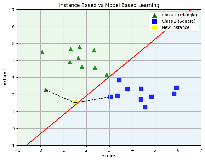
Instance Based vs Model Based
Training Mode
Another classification method is based on how ML system can be trained.
Batch Learning
Batch learning systems can be trained using all the data in batches. The system generally cannot learn incrementally and training is compute intensive. Such systems must be trained off-line and then deployed in production for inference.
Online Learning
An online system can learn incrementally using data-sample or mini-batches. The data itself does not need to be retained as learning is assimilated in the model. Online systems can also learn on huge data sets often which cannot fit single computers memory. Such learning is known as out-of-core learning. One important parameter of such system is learning rate, i.e. how fast you adapt your system in response to new data, or how much you forget the old data. As you can imagine this obviously poses challenge, as bad data can cause model drift.
Deployment Context
ML models can be deployed in the cloud, on edge devices, or in hybrid systems. Cloud ML handles large datasets and complex models, while Edge ML / TinyML runs lightweight models locally for low latency, privacy, and reduced bandwidth usage. Hybrid systems may combine signal processing (SP) for pre-processing with ML for prediction, which improves performance and reduces computational load on constrained devices.
Main Challenges of ML
There is a famous saying in ML Systems community: "Garbage in Garbage out", there are two fundamental issues one can run into when dealing with ML systems:
- Poor quality of data;
- Poor quality of model.
These two further translate into several challenges, e.g., class imbalance, biased models, and irrelevant feature selection. We will briefly touch upon these to develop deeper understanding.
Data
Sufficiency of Data
In machine learning, data sufficiency refers to the availability of a dataset that is large and representative enough for a model to learn the underlying distribution of the problem domain. When data are sufficient, the model can generalize well to unseen samples, achieve stable convergence during training, and ensure that all relevant input features and conditions are adequately represented.
From a statistical standpoint, sufficiency is related to the classical notion of a sufficient statistic, which captures all the information in the data that is relevant to the estimation of a parameter (Fisher, 1922 [1]). In learning theory, sufficiency is often characterized through the convergence of empirical risk to expected risk. Specifically, for a hypothesis trained on a dataset, we desire that:
where denotes the empirical risk computed on the training data, and is the expected risk over the true data distribution. The inequality expresses that with sufficient data, empirical performance approximates true performance with high probability.
When data are insufficient in quantity, diversity, or representativeness, the model fails to capture the true structure of the problem. Insufficient data can result in:
- Overfitting, where the model memorizes noise instead of learning generalizable patterns;
- High variance, producing unstable performance across different training runs;
- Poor generalization, yielding low accuracy on unseen data;
- Systematic bias, especially when minority groups or rare cases are underrepresented.
These effects are amplified in high-dimensional spaces, where the curse of dimensionality implies that the number of samples required for accurate learning grows exponentially with the number of input features. Regularization, transfer learning, and data augmentation can partially mitigate, but not eliminate, insufficiency effects.
The phrase “The Unreasonable Effectiveness of Data” was introduced by Halevy, Norvig, and Pereira (2009), inspired by Eugene Wigner’s essay “The Unreasonable Effectiveness of Mathematics in the Natural Sciences.” The authors observed that simple models trained on massive and diverse datasets can outperform complex models trained on smaller, curated datasets.
The core insight is that increasing the quantity and diversity of data can compensate for model simplicity. Empirical evidence from large-scale machine learning and deep learning supports this phenomenon, where performance continues to improve predictably with more data.
Key Implications:
- Redundant but diverse data provides richer coverage of latent factors.
- Model capacity and data scale are complementary resources.
- Empirical scaling laws demonstrate predictable performance improvements with increased data and compute.
Modern ML theory increasingly recognizes data—not algorithms—as the primary driver of performance. Several frameworks describe this shift.
Data Scaling Laws
Empirical studies [3][4] demonstrate that model performance scales predictably with compute and data size :
where and are empirically derived exponents. This relationship formalizes how larger datasets consistently yield measurable improvements, given sufficient model capacity.
Data-Centric AI
Proposed by Andrew Ng [5], data-centric AI emphasizes improving data quality—rather than model complexity—as the main driver of progress. It advocates for consistent labeling, representativeness, and transparency in data collection and curation.
Foundation Models and Data Governance
The emergence of large pretrained foundation models (e.g., GPT, CLIP) trained on web-scale data highlights both the power and the risks of massive datasets. Issues of bias, provenance, and ethical data curation are now central to the responsible development of AI systems.
Model and Features
The second core issue is with regards to features and how model learns from the data. The model can only learn to generalise if trained with relevant features, exposing models to irrelevant features can lead to poor models. Feature Engineering, i.e. careful selection of input features for ML problems therefore forms fundamental step in developing good ML Systems. Often feature engineering, also involves combination of features to arrive at the new feature which can represent the data much better. This is known as feature extraction. For instance, one can think of extracting change points in signals, frequency domain features or dimensionality reduction techniques which can generate new features for the model.
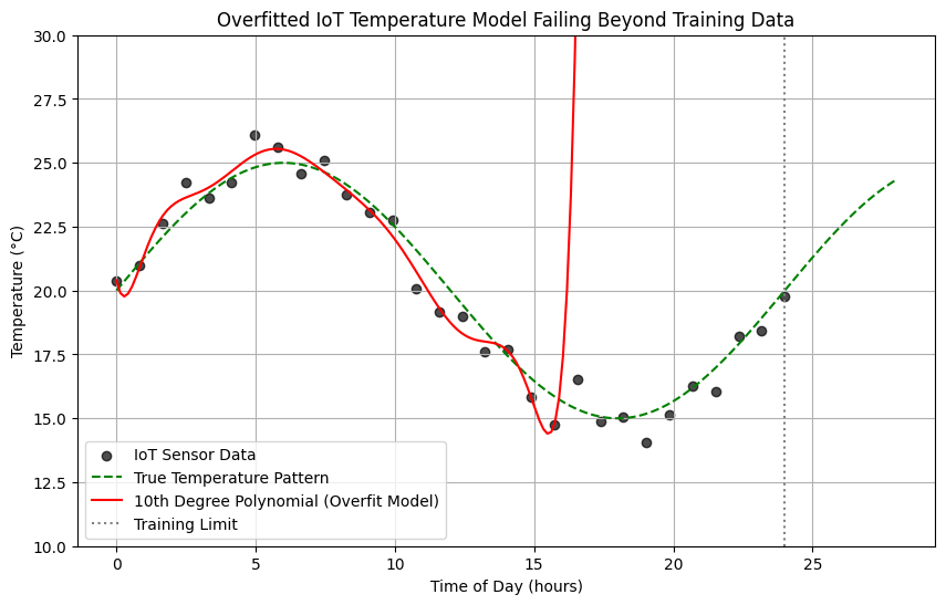
Overfitting the Training Data
One of the core issues with ML models can be their sensitivity to zoom in on the smaller variations. This could lead to the issue of assuming over-generalisation of a trend which is an outlier. In other words, if a model becomes too flexible or is trained too long, it may start to memorize the training examples rather than learning the true underlying patterns. This phenomenon is called overfitting.
Definition
A model is said to overfit when it performs very well on the training data but poorly on new, unseen data, essentially it has learned the noise instead of the signal.
Reasons for Overfitting
Overfitting becomes more likely when:
- The model has high capacity, i.e., too many parameters or too flexible a structure (e.g., deep neural networks, large decision trees).
- The dataset is small or noisy, i.e., the model mistakes random fluctuations for structure.
- The training process is excessive, i.e., the model continues optimizing until it starts chasing noise.
- No constraints are placed on learning, i.e., all patterns, even spurious ones, are given equal importance.
Example
Overfitting through lens of IoT case-study
Suppose you are building an IoT system to predict the indoor temperature using data from sensors that measure:
- Outdoor temperature
- Humidity
- Time of day
- HVAC (air conditioning) status
You train a machine learning model using one week of sensor data. A good model will learn core trends e.g.
- Temperature drops at night
- HVAC usage lowers temperature
- Humidity slightly affects readings
This model performs well on both training and new data from the next week.
If the model is too complex (e.g., a deep neural network with too many parameters or decision trees with too many branches), it might learn:
- The exact sensor noise patterns on specific days
- Unnecessary correlations (e.g., “temperature always rises at 2:03 PM” because of one-time sensor drift)
Now, when new data arrives (next week’s sensor readings), these patterns don’t hold true — the model gives inaccurate predictions. This is an example of overfitting.
Regularisation
Constraining a model to make it simpler and reduce the risk of overfitting is called regularisation. Imagine we have a network of IoT sensors measuring temperature in a building. The raw data may have fluctuations due to random noise, sensor errors, or temporary events, in addition to genuine trends.
Think of a model predicting temperatures from IoT sensors like a thermostat trying to adjust a building’s heating. If it reacts to every tiny blip in the sensor readings, it would constantly turn the heating up and down, making the system unstable. Regularization acts like a gentle rule saying, “Only respond to consistent trends, not every tiny spike.” This way, the model focuses on the real patterns in the data, ignoring random noise, and gives smoother, more reliable temperature predictions—just like a smart thermostat keeping the building comfortably warm without overreacting to every draft.
The amount of regularisation you apply to the model is controlled via hyper-parameter. The hyper-parameter tunning therefore is an art which a good ML engineer can master by having deeper theoretical understanding.
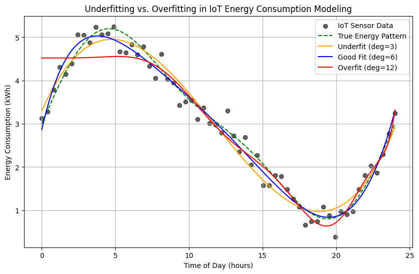
Underfitting the Training Data
Underfitting occurs when a model is too simple to capture the underlying patterns in the data. It fails to perform well even on the training data, not just new data, because it cannot represent the complexity of the relationships in the dataset.
Underfitting through lens of IoT case-study
In the context of IoT temperature data, underfitting might happen if the model is too rigid—for example, if it only predicts a single constant value for all times, ignoring trends like daily temperature cycles or seasonal changes. The predictions would consistently miss important variations, resulting in large errors.
Reasons for Underfitting
- Model is too simple: The structure of the model cannot capture the real patterns (e.g., using a very basic rule for a complex signal).
- Insufficient features or input information: The model does not have enough relevant inputs to make accurate predictions.
- Excessive regularization: Constraining the model too much can force it to ignore important patterns.
Definition
In short, underfitting is like trying to summarize a novel with a single word—the model is too limited to capture the important details.
Bias vs Variance Tradeoff
In supervised learning, understanding the bias-variance tradeoff is crucial to building models that generalize well. The total expected error of a model can be decomposed as:
Where:
- is the true output,
- is the prediction of the model,
- is the irreducible error (noise in the data),
- measures how much the average model prediction differs from the true function ,
- measures how much predictions vary for different training datasets.
Tradeoff Intuition
- High bias: The model is too simple (underfitting). It cannot capture important patterns, leading to systematic errors. Example: predicting IoT temperatures as a constant value.
- High variance: The model is too complex (overfitting). It reacts to random fluctuations in the training data, producing unstable predictions across datasets. Example: predicting temperature by memorizing every spike from a small sensor dataset.
The goal is to find a balance: a model complex enough to capture meaningful patterns, but simple enough to generalize well to unseen data.
Training and Validation of Models
When developing any model, it is important to evaluate its performance properly to ensure it works well on new, unseen data. This involves dividing the data or observations into training and validation sets.
Training Set
The training set is used to adjust the model’s internal parameters. The model learns patterns or structures from this data, optimizing itself to reduce error or improve performance on the training observations.
Validation Set
The validation set is kept separate from training. It is used to check how well the model generalizes. If a model performs well on the training data but poorly on the validation set, it indicates overfitting, meaning the model has learned details specific to the training set rather than general patterns.
Why Cross-Validation is Required
Splitting the dataset into just one training set and one validation set has a major drawback: the performance estimate can depend heavily on how the split was done. Some splits may be easier to predict than others, giving misleading results.
Cross-validation solves this problem by repeating the training/validation process multiple times with different splits. This way, every observation gets used for both training and validation, producing a more reliable and less biased estimate of the model’s performance. It also helps detect whether the model is stable across different subsets of data.
Optimal Splits
Choosing the right proportion for training and validation sets is important. Common splits are 70/30 or 80/20, where the larger portion is used for training. If the training set is too small, the model may underfit because it does not have enough data to learn the patterns. If the validation set is too small, performance estimates may have high variance and may not reliably reflect the model’s generalization ability.
Cross-validation effectively mitigates this problem by allowing all data points to be part of both training and validation sets in different iterations. This reduces dependency on a single split and improves the robustness of performance evaluation.
Cross-Validation Procedure
-
Divide the dataset into roughly equal parts (folds).
-
For each fold:
- Train the model on folds.
- Validate it on the remaining fold.
-
Repeat times, each time using a different fold for validation.
-
Average the results to obtain a final performance measure.
References
[1] R. A. Fisher, On the Mathematical Foundations of Theoretical Statistics, Philosophical Transactions of the Royal Society of London. Series A, Containing Papers of a Mathematical or Physical Character, Vol. 222 (1922), pp. 309-368, 1922
[2] Halevy, A., Norvig, P., & Pereira, F. "The Unreasonable Effectiveness of Data.", IEEE Intelligent Systems, 24(2), 8–12., 2009
[3] Kaplan, J. et al. Scaling Laws for Neural Language Models. arXiv:2001.08361. , 2020
[4] Hoffmann, J. et al. Training Compute-Optimal Large Language Models. arXiv:2203.15556., 2025
[5] Ng, A. MLOps: From Model-Centric to Data-Centric AI. DeepLearning.AI Blog., 2021